EARTHQUAKE ENGINEERING AND STRUCTURAL DYNAMICS Earthquake Engng Struct. Dyn. 2002; IN PRINT :1–23 Prepared using eqeauth.cls [Version: 2002/11/11 v1.00]
Time Domain Simulation of Soil–Foundation–Structure Interaction in non–Uniform Soils Boris Jeremi´c1∗ , Guanzhou Jie2 , Matthias Preisig3 , Nima Tafazzoli4 1
4
Department of Civil and Environmental Engineering, University of California, One Shields Ave., Davis, CA 95616, Email:
[email protected] 2 Wachovia Corporation, 375 Park Ave, New York, NY, 3 Ecole Polytechnique F´ ed´ erale de Lausanne, CH–1015 Lausanne, Switzerland, Department of Civil and Environmental Engineering, University of California, One Shields Ave., Davis, CA 95616,
key words:
Time Domain, Earthquake Soil–Foundation–Structure Interaction, Parallel Computing SUMMARY
Presented here is a numerical investigation of the influence of non–uniform soil conditions on a prototype concrete bridge with three bents (four span) where soil beneath bridge bents is varied between stiff sands and soft clay. A series of high fidelity models of the soil–foundation–structure system were developed and described in some details. Development of a series of high fidelity models was required to properly simulate seismic wave propagation (frequency up to 10 Hz) through highly nonlinear, elastic plastic soil, piles and bridge structure. Eight specific cases representing combinations of different soil conditions beneath each of the bents are simulated. It is shown that variability of soil beneath bridge bents has significant influence on bridge system (soil-foundation-structure) seismic behavior. Results also indicate that free field motions differ quite a bit from what is observed (simulated) under at the base of the bridge columns indicating that use of free field motions as input for structural only models might not be appropriate. In addition to that, it is also shown that usually assumed beneficial effect of stiff soils underneath a structure (bridge) cannot be generalized and that such stiff soils do not necessarily help seismic performance of structures. Moreover, it is shown that dynamic characteristics of all three components of a triad made up of of earthquake, soil and structure play crucial role in determining the seismic performance of the infrastructure (bridge) system. c 2002 John Wiley & Sons, Ltd. Copyright
1. Introduction Currently, for a vast majority of numerical simulations of the response of bridge structures to seismic ground motions, the input excitations are defined either from a family of damped
∗ Correspondence
to: Boris Jeremi´ c, Department of Civil and Environmental Engineering, University of California, One Shields Ave., Davis, CA 95616, Email:
[email protected] Contract/grant sponsor: NSF–CMS; contract/grant number: 0337811
c 2002 John Wiley & Sons, Ltd. Copyright
Received May 2008 Revised October 2008 Accepted December 2008
2
´ B. JEREMIC
response spectra or as one or more time histories of ground acceleration. These input excitations are usually applied simultaneously along the entire base of the structure, regardless of its dimensions and dynamic characteristics, the properties of the soil material in foundations, or the nature of the ground motions themselves. Application of ground motions like this does not account for spatial variations of the traveling seismic waves that control the ground shaking. In addition to that, ground motions applied in such a way neglect the soil–structure interaction (SSI) effects, that can significantly change ground motions that are actually developing in such SSI system. A number of papers in recent years have investigated the influence of the SSI on behavior of bridges. Even though interest in SSI effects has grown significantly in recent years, Tyapin (2007) notes that after four decades of intensive studies there still exists a large gap in SSI simulation tools used between SSI specialists and practicing civil engineers. Results obtained using specialized SSI simulation tools match closer experimental and field data (validate better (Oberkampf et al., 2002)) than regular, general simulation tools. There is therefor a significant need to transfer advanced simulation technology (numerical tools, education...) to practicing engineers, so that SSI effects can be appropriately taken into account in designing structures. One of the first studies that has developed a three-dimensional, nonlinear model for complete soil – skew highway bridge system interacting with their surrounding soils during strong motion earthquakes was done by Chi Chen and Penzien (1977). Due to a limitations of computer power, a number of studies were conducted with a variety of modeling simplifications that usually rely on closed form solutions for elastic material. We mention few such studies below. Makris et al. (1994) developed a simple integrated procedure to analyze soil-pile foundation-superstructure interaction, based on dynamic impedance and kinematic seismic response factors of pile foundations with a simple six-degree-of-freedom structural model. Sweet (1993) approximated geometry of pile groups to perform finite element analysis of a bridge system subjected to earthquake loads, while Dendrou et al. (1985) resorted to combining finite element and boundary integral methodology to resolve seismic wave propagation from soil to bridge structure. It is very important to note that assumed beneficial role of not performing a full SSI analysis has been turned into dogma, particularly since the NEHRP-94 seismic code states that: ”These [seismic] forces therefore can be evaluated conservatively without the adjustments recommended in Sec. 2.5 [i.e. for SSI effects]”. A number of studies have therefor investigated importance of performing SSI analysis. McCallen and Romstadt (1994) developed a detailed, 3D numerical simulation of dynamic response of a short-span overpass bridge system and showed that even when structure remains elastic, the complete soil–structure system is highly nonlinear due to soil interaction. SSI effects on cable stayed bridges together with effects of foundation depth were investigated by Zheng (1995). Gazetas and Mylonakis (1998) and Mylonakis et al. (2006) emphasized importance of proper SSI analysis on response of bridges and provided important insight on failure of Hanshin Expressway bridge during Kobe earthquake. Small (2001) developed SSI models showing how use of simple spring models for the soil behavior could lead to erroneous result and recommended that their use should be discontinued. In addition to that, they showed that the type of structure and its stiffness could have an effect on the deformation of the foundation. Tongaonkar and Jangid (2003) investigated SSI effects on peak response of three-span continuous deck bridge seismically isolated by the elastomeric bearings and found that bearing displacements at abutment locations may be underestimated if the SSI effects are not considered. Chouw and Hao (2005) studied the effect of spatial c 2002 John Wiley & Sons, Ltd. Copyright :1–23 Prepared using eqeauth.cls
Earthquake Engng Struct. Dyn. 2002;
IN PRINT
TIME DOMAIN SFSI IN NON–UNIFORM SOILS
3
variations of ground motion with different wave propagation apparent velocities in soft and medium stiff soil, and revealed significant SSI effects. In addition to that, it was found that non-uniform ground excitation effects are significant, especially when a big difference between the fundamental frequency of the bridge frames and the dominant frequencies of the ground motions exists. Soneji and Jangid (2008) analyzed influence of dynamic SSI on behavior of seismically isolated cable-stayed bridge and observed that the soil had significant effects on the response of the isolated bridge. In addition to that, inclusion of SSI was found to be essential for effective design of seismically isolated cable-stayed bridge, especially when the towers are very rigid and the soil is soft to medium stiff. Elgamal et al. (2008) performed a very advanced 3D analysis of a full soil–bridge system, focusing on interaction of liquefied soil in foundation and bridge structure. In addition to studies showing importance of SSI analysis, beneficial (as suggested by the code) and possibly detrimental effects of SSI were analyzed in a number of studies. For example Kappos et al. (2002) found that there are advantages in including SSI effects in the seismic design of irregular R/C bridges as seismic forces are typically lower when SSI is included in the analysis. This conclusion nicely reinforces recommendation of NEHRP-94 seismic code, mentioned above. On the other hand, Jeremi´c et al. (2004) found that SSI can have either beneficial or detrimental effects on structural behavior and is dependent on the dynamic characteristics of the earthquake motion, the foundation soil and the structure. Main conclusion was that while in some cases SSI can improve overall dynamic behavior of structural system, there are many cases where SSI is detrimental to such overall seismic response of the soil–structure system. However, due to computational limitations, Jeremi´c et al. (2004) had to analyze soil–pile system separately from the structure, thus reducing modeling accuracy. Present paper significantly improves on modeling, treating complete earthquake–soil–bridge system as tightly coupled triad, where interacting components (dynamic characteristics of the earthquake, soil and the bridge structure) control seismic response. Based on the above (limited) literature overview, it seems that importance of full SSI analysis is well established in the research community. Purpose of this paper is to present a methodology for high fidelity modeling of seismic soil–structure interaction. This is done in Section 2. Presented methodology relies on rational mechanics and aims to reduce modeling uncertainty, by employing currently best available models and simulation procedures. In addition to presenting such state–of–the–art modeling, simulation results are used to illustrate influence of non–uniform soils on seismic response of a prototype bridge system. A number of interesting and sometimes perhaps counter-intuitive results, given in Section 3, emphasize the need for a full, detailed SSI analysis for each particular Earthquake–Soil–Structure triad. Analyzed bridge model represents prototype model that was devised as part of a grand challenge, pre–NEESR project, funded by NSF NEES program. Pre–NEESR project, titled ”Collaborative Research: Demonstration of NEES for Studying Soil-Foundation-Structure Interaction” (PI Professor Wood from UT) brought together researchers from University of California at Berkeley, University of Texas at Austin, University of Nevada at Reno, University of Washington, University of Kansas, Purdue University and University of California at Davis, with the aim of demonstrating use of NEES facilities and use of existing and development of new simulations tools for studying SSI problems. Presented modeling, simulations and developed parallel simulations tools (used here and described by Jeremi´c and Jie (2007, 2008)) represented a small part of this large and ambitious project. c 2002 John Wiley & Sons, Ltd. Copyright :1–23 Prepared using eqeauth.cls
Earthquake Engng Struct. Dyn. 2002;
IN PRINT
´ B. JEREMIC
4
2. Model Development and Simulation Details The finite element models used in this study have combined both solid elements, used for soils, and structural elements, used for concrete piles, piers, beams and superstructure. In this section described are material and finite element models used for both soil and structural components. In addition to that, described is the methodology used for seismic force application and staged construction of the model, followed by a brief description of a numerical simulation platform used for all simulations presented here. 2.1. Soil Model Two types of soil were used in modeling. First type was based on soil found at the Capitol Aggregates site, a local quarry located south–east of Austin, Texas. This soil was chosen as part of modeling requirement for above mentioned pre–NEES project. Site characterization has been preformed to collect information on soil by Kurtulus et al. (2005). Based on stress-strain curve obtained from a triaxial test (Kurtulus et al., 2005), as shown in Figure 1(a), a nonlinear, kinematic hardening, elastic-plastic soil model has been developed using Template Elastic plastic framework (Jeremi´c and Yang, 2002). It should be noted that an isotropic hardening model would have been enough to fit monotonic lab test data. However, for cyclic loading, only kinematic hardening (in this case, rotational kinematic) is able to appropriately model Bauschinger effect. Developed model consists of a DruckerPrager yield surface, Drucker–Prager plastic flow directions (potential surface) and a nonlinear Armstrong-Frederick (rotational) kinematic hardening rule (Armstrong and Frederick, 1966). Model calibration was performed using limited data set resulting in a very good match (see Figure 1(b)). Initial opening of a Drucker–Prager cone was set at approximately 5o only (in
a)
b)
Figure 1. (a) Stress–strain curve obtained from triaxial compression test (b) Stress–strain curve by obtained by calibrated model (from Depth 10.6f t)
normal–shear stress space). This makes for a very sharp Drucker–Prager cone, with a very small elastic region (similar to Dafalias Manzari models Dafalias and Manzari (2004)). The actual deviatoric hardening is produced using Armstrong–Frederick nonlinear kinematic hardening with hardening constants a = 116.0 and b = 80.0. c 2002 John Wiley & Sons, Ltd. Copyright :1–23 Prepared using eqeauth.cls
Earthquake Engng Struct. Dyn. 2002;
IN PRINT
TIME DOMAIN SFSI IN NON–UNIFORM SOILS
5
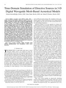
Second type of soil used in modeling was soft clay, Bay Mud). This type of soil was modeled using a total stress approach with an elastic perfectly plastic von Mises yield surface and plastic potential function. The shear strength for such (very soft) Bay Mud material was chosen to be Cu = 5.0 kPa (Dames and Company, 1989). Since this soil is treated as fully saturated and there is not enough time during shaking for any dissipation to occur, elastic–perfectly plastic model provides enough modeling accuracy. Soil Element Size Determination The accuracy of a numerical simulation of seismic wave propagation in a dynamic Soil-Structure–Foundation Interaction) (SFSI) problems is controlled by two main parameters Preisig (2005): 1. The spacing of nodes in finite element model ∆h 2. The length of time step ∆t. Assuming that numerical method converges toward exact solution as ∆t and ∆h tend toward zero, desired accuracy of solution can be obtained as long as sufficient computational resources are available. In order to represent a traveling wave of a given frequency accurately about 10 nodes per wavelength are required. Fewer than 10 nodes can lead to numerical damping as discretization misses certain peaks of seismic wave. In order to determine appropriate maximum grid spacing the highest relevant frequency fmax that is present in model needs to be found by performing a Fourier analysis of input motion. Typically, for seismic analysis one can assume fmax = 10Hz. By choosing wavelength λmin = v/fmax , where v is (shear) wave velocity, to be represented by 10 nodes, smallest wavelength that can still be captured with any confidence is λ = 2∆h, corresponding to a frequency of 5fmax . The maximum grid spacing should therefor not be larger than v λmin (1) = ∆h ≤ 10 10fmax where v is smallest wave velocity that is of interest in simulation (usually wave velocity of softest soil layer). In addition to that, mechanical properties of soil changes with (cyclic) loadings as plastification develops. In order to quantify those changes in soil stiffness, a number of laboratory and in situ tests were performed by Kurtulus et al. (2005). Moduli reduction curve (G/Gmax ) and damping ratio relationship were then used to capture determine soil element size while taking into account soil stiffness degradation (plastification). Using shear wave velocity relation with shear modulus s G (2) vshear = ρ one can readily obtain dynamic degradation of wave velocities. This leads to smaller element size required for detailed simulation of wave propagation in soils which have stiffness degradation (plastification). The addition of stiffness degradation effects (plastification) of soil on soil finite size are listed in Table I. Based on above soil finite element size determination, a three bent prototype finite element model has been developed and is shown in Figure 2. The model features 484,104 DOFs, 151,264 soil and beam–column elements, it is intended to model appropriately seismic waves of up to 10Hz, for minimal stiffness degradation of c 2002 John Wiley & Sons, Ltd. Copyright :1–23 Prepared using eqeauth.cls
Earthquake Engng Struct. Dyn. 2002;
IN PRINT
´ B. JEREMIC
6
Table I. Soil finite element size determination with shear wave velocity and stiffness degradation effects for assumed seismic wave with fmax =10 HZ, (minimal value of G/Gmax corresponding to 0.2% strain level.)
Depth (f t) 0 1 2.5 7 14 21.5 38.5
Layer thick. (f t) 1 1.5 4.5 7 7.5 17 half-space
vs (f ps) 320 420 540 660 700 750 2200
G/Gmax 0.36 0.36 0.36 0.36 0.36 0.36 0.36
vsmin (fps) 192 252 324 396 420 450 1320
∆hmax (f t) 1.92 2.52 3.24 3.96 4.20 4.50 13.20
Figure 2. Detailed Three Bent Prototype SFSI Finite Element Model, 484,104 DOFs, 151,264 Elements.
G/Gmax = 0.08, maximum shear strain of γ = 1% and with maximal element size ∆h = 0.3 m. It is noted that even larger set of models was created, that was able to capture 10 Hz motions, for G/Gmax = 0.02, and maximum shear strain of γ = 5%. This (our largest to date) set of models features over 1.6 million DOFs and over half a million finite elements. However, results from this very detailed model were almost same as results for model with half a million DOFs (484,104 to be precise) and it was decided to continue analysis with this smaller model. However, development of this more detailed model (featuring 1.6 million DOFs), that did not add much (anything) to our results brings another very important issue. It proves very important to develop a hierarchy of models that will, with refinement, improve our simulations. When model refinements (say mesh refinement) does not improve simulation results any more c 2002 John Wiley & Sons, Ltd. Copyright :1–23 Prepared using eqeauth.cls
Earthquake Engng Struct. Dyn. 2002;
IN PRINT
TIME DOMAIN SFSI IN NON–UNIFORM SOILS
7
(there is no observable difference), model can be considered mature (Oberkampf et al., 2002) and no further refinement is necessary. This maturation of model allows us use of immediate lower level (lower level of refinement) model for production simulations. It is therefore always advisable to develop a hierarchy of models, and to potentially settle for model that is one level below the most detailed model. This most detailed models is chosen as model which did not improve accuracy of simulation significantly enough to warrant its use. For our particular example, the most detailed model used, did not improve results (displacements, moments...) significantly (actually it almost did not change them at all) implying that accurate modeling of frequencies up to 10 Hz for this Earthquake–Soil–Structure system did not affect seismic response. Time Step Length Requirement The time step ∆t used for numerically solving nonlinear vibration or wave propagation problems has to be limited for two reasons (Argyris and Mlejnek, 1991). The stability requirement depends on time integration scheme in use and it restricts the size of ∆t = Tn /10. Here, Tn denotes smallest fundamental period of the system. Similar to spatial discretization, Tn needs to be represented with about 10 time steps. While accuracy requirement provides a measure on which higher modes of vibration are represented with sufficient accuracy, stability criterion needs to be satisfied for all modes. If stability criterion is not satisfied for all modes of vibration, then the solution may diverge. In many cases it is necessary to provide an upper bound to frequencies that are present in a system by including frequency dependent damping to time integration scheme. The second stability criterion results from the nature of finite element method. As a wave front progresses in space, it reaches one point (node) after the other. If time step in finite element analysis is too large, than wave front can reach two consecutive points (nodes) at the same time. This would violate a fundamental property of wave propagation and can lead to instability. The time step therefore needs to be limited to ∆t