IEEE SIGNAL PROCESSING LETTERS, VOL. 14, NO. 9, SEPTEMBER 2007
585
Time-Multiplexed Training for Time-Selective Channels Zijian Tang and Geert Leus
Abstract—Pilot-assisted channel estimation is considered in this letter, where the channel is assumed to be time-selective and can be accurately fit by a basis expansion model. The position and power of the pilots are crucial to the mean square error of the channel estimator. In this paper, we present nonlinear integer programming algorithms to optimize the position and power of the pilots. In comparison with the traditional equi-distant/powered pilot structure, the solution obtained from the proposed algorithms yields a better performance. Index Terms— Basis expansion model (BEM), pilot-assisted channel estimation, time-selective channels.
I. INTRODUCTION ECENTLY, parsimonious channel models to track the channel’s time variation have drawn increasing attention. One of the approaches, known as the basis expansion model (BEM) will be treated in this letter. Examples of such BEMs are the complex exponential BEM (CE-BEM) [1]–[4], the polynomial BEM (P-BEM) [5], the discrete prolate spheroidal BEM (DPS-BEM) [6], etc. Note that the CE-BEM in [2], [4] is slightly different than that in [1], [3]: the former is sometimes referred to as the critically-sampled CE-BEM [(C)CE-BEM] because the BEM period equals the window length, whereas the latter uses a longer period and is thus also referred to as the oversampled CE-BEM [(O)CE-BEM]. Based on a certain BEM assumption, time-selective channel estimation reduces to estimating the BEM coefficients. We focus on pilot-assisted channel estimators corresponding to different BEM assumptions using time-multiplexed (TM) training, i.e., pilots are inserted in the time-domain as considered in [2], [4]–[6]. Usually, the total number of pilots (bandwidth constraint) as well as the total power (power constraint) is limited. The question arises as to what will be the optimal pilot structure (positions and powers). Note that the optimal pilot structure will depend on both the optimality criterion and the considered BEM. For instance, in terms of the maximum BEM modeling error and under the P-BEM assumption, the optimal pilot positions correspond to the roots of the Chebyshev polynomials [7]. In this letter, we will not consider the influence of the BEM modeling error, which can be kept very small in most practical situations [6], and take the channel mean square error
R
Manuscript received October 19, 2006; revised January 17, 2007. This work was supported in part by NWO-STW under the VICI program (DTC.5893) and the VIDI program (DTC.6577). The associate editor coordinating the review of this manuscript and approving it for publication was Dr. Gerald Matz. The authors are with Delft University of Technology-Fac. EEMCS, 2628 CD Delft, The Netherlands (e-mail:
[email protected];
[email protected]). Color versions of one or more of the figures in this paper are available online at http://ieeexplore.ieee.org. Digital Object Identifier 10.1109/LSP.2007.896146
(MSE) as the optimality criterion. It is shown in [2], [4] that for the (C)CE-BEM, the optimal pilots must be uniformly distributed with equal power.1 However, it is not yet clear what the optimal pilot structure is for other BEMs, e.g., the DPS-BEM, the P-BEM or the (O)CE-BEM, which are of more practical significance in view of their superior modeling capacity [6]. In this letter, we will optimize the TM training scheme under a general BEM assumption. An MSE-related cost function will be formulated for the LS channel estimator, and translated into a mixed-integer non-linear programming problem [8]. We show that the resulting optimal pilot structure can produce a lower channel MSE than the classical equi-distant/powered pilots if a general BEM assumption is adopted. Notation: We use upper (lower) bold face letters to de, and represent note matrices (column vectors). conjugate, transpose and complex conjugate transpose (Hermitian), respectively. stands for an identity matrix. stands for a diagonal matrix with as its diagonal, and for a block-wise diagonal matrix with as its diagonal blocks. represents the trace of . Further, we use to indicate the st entry of the matrix , and to indicate the st row of . II. DATA MODEL FOR TIME-SELECTIVE CHANNEL ESTIMATION Let us consider a communication system over a time-selective channel. The I/O relationship in discrete form can be expressed , where , , and denote respecas tively the received signal, the transmitted signal and the noise stands for the “true” channel gain, at the th time instant; which varies with time for . To approximate this time-variation with a BEM, let us choose the time instants as an observation window and collect all the channel gains within this observation window in the vector . By selecting a proper scale for the BEM, we can closely fit the channel’s time variation within BEM coefficients the observation window with (1) BEM matrix, and a -long where is an vector containing the related BEM coefficients. represents the BEM modeling error. With its entries independent of to the channel, a BEM reduces the system scale from at the price of a modeling error, which is nonetheless 1The optimal pilots proposed in [2], [4] are based on a linear minimum mean square error estimator under certain statistical assumptions, but the optimality remains also valid for the least squares (LS) estimator. We will deal with an LS estimator since it is more robust to a possible mismatch in the channel statistics.
1070-9908/$25.00 © 2007 IEEE
586
IEEE SIGNAL PROCESSING LETTERS, VOL. 14, NO. 9, SEPTEMBER 2007
ignored in this paper for the design of the channel estimator. This is because the modeling error can be kept very small by choosing an appropriate BEM [6]. As a result, its impact at a practical signal-to-noise ratio (SNR) can be almost neglected. Furthermore, it is usually difficult to gauge the modeling error when the channel itself is unknown. We also note that the idea of a BEM is reflected in some other applications without inducing a modeling error, e.g., the frequency-domain channel in an OFDM system [9] can be model by a (C)CE-BEM whereas the frequency-domain channel in an OFDM system with virtual subcarriers [10] can be modeled by an (O)CE-BEM. For these cases, the approach discussed in this letter can be also applied. To estimate the BEM coefficients , we resort to a TM training scheme, in which the pilots and the data will be pilots interleaved in the time domain. Suppose there are transmitted during the observation window, whose positions are . Furthermore, we collected in the set has phase and power , i.e., assume that the th pilot with the total power for training . With the aid of these notations and neglecting the modeling error, we can express the I/O relationship that results from the pilots in matrix/vector form as
Fig. 1. Flowchart of GA.
and , the primal problem becomes simply the search for the subject to a fixed , and the relaxed master problem optimal becomes the search for the optimal subject to a fixed . We summarize the GBD algorithm as follows. 1) Let the superscript denote the iteration index. To initialize, set , and assume and
(2) is a vector collecting the received samples where ; at the pilot-related positions, i.e., is similarly defined as ; and are both diagonal matrices with and as their diagonals, respectively; is a matrix consisting of rows carved out of corresponding to the pilot positions. An LS estimate from (2) can be obtained as resulting in a channel MSE equal to . Assuming the to be white with variance , we can express the MSE noise as (3) From the above, we remark that the phase of the pilots has no impact on the channel MSE, and we only need to focus on the powers and positions of the pilots. The optimization problem can thus be formulated as
(4) (5)
III. OPTIMIZATION ALGORITHM The above formulation is a mixed-integer non-linear optimization problem, where we have posed restrictions on the total number and power of the pilots. [8] provides an algorithm known as the generalized Benders decomposition (GBD). In a nutshell, the GBD iteratively projects the minimization problem —(primal problem) and the —(relaxed master onto the problem). Since the constraints in (4) and (5) are separable in
. 2) For
, solve
(4) resulting in 3) For , solve
subject to .
to (5) resulting in . 4) For a predetermined , if terminate. Otherwise, set
subject
then and return to Step 2.
The primal problem at Step 3 is a nonlinear programming problem (NLP), which can be solved analytically if [10]. In other cases where , we can resort to the . The solution correMATLAB built-in function sponds to the global optimum due to the following lemma. Lemma 1: The function is strictly convex on the positive diagonal matrix for a given . To prove the above lemma, we realize that the function is strictly convex on a positive-definite Hermitian matrix [11]. In our case, is linear in for a given , which preserves the convexity. However, the master problem at Step 2, which is essentially a binary programming problem, is more problematic. Especially due to the fact that the MSE is not a convex function on the pilot positions despite Lemma 1. In [12] and [13], this is solved by relaxing the binary problem to a non-binary problem such that the convexity can be still called upon. Unfortunately, this approach, when applied to our problem, does not facilitate a fast convergence due to a very large pilot position space. In this letter, we resort to a combined genetic algorithm (GA) [14], whose working principle is illustrated by the flowchart in Fig. 1, with: • “Population” representing a set of candidate (pilot position) solutions. • “Weakness” representing the cost function value defined in (3) for each candidate. Those candidates that do not satisfy
TANG AND LEUS: TM TRAINING FOR TIME-SELECTIVE CHANNELS
condition (4) will be penalized by a weakness value equal to infinity. • “Reproduction” representing the operation that copies the population except for the candidates that either have the largest weakness or the smallest weakness. The former will be discarded while the latter will be copied twice since it has the lowest MSE at the moment. • “Crossover” representing the operation applied on the candidate pool produced by the reproduction: at the th iteration, all the candidates are randomly grouped into pairs (parents). Let us take one such pair for example: suppose “Parent1” is the th candidate and “Parent2” the th candidate with . Here, stands in our context for the position of the th pilot that corresponds to the th candidate obtained at the th iteration. “Mating” these two parents results in two new candidates (children) with “Child1” and “Child2” as denoted as . In generating each entry of the children, either of two operations will take place: replication or swapping with a probability of 0.5, respectively. For the th entry for instance, in case of replication , and . In case of swapping, we first express the th entry of “Parent1” and “Parent2” in binary-form. These two binary strings are then divided at the same arbitrary place, from which the right-hand part of “Parent2” will be concatenated to the left-hand part of “Parent1” and vice versa. In this way, two new binary strings are created and converted back in decimal form.2 If the observation window size or pilot number is large, the GA must abide with a large population size. This results in a higher complexity and lower convergence rate, which in practice, often leads to a “near-optimal” solution. It is thus helpful if we could equip the GA with some a priori knowledge about the solution. For the considered case (both and are assumed to be even), we could constrain the pilot structure to be symmetric with respect to the center of the observation window, e.g., we let and . This constraint is introduced due to the following properties. Property 1: Without loss of generality, we can design the BEM in a particular way. For the CE-BEM, we take , where for the (C)CE-BEM as in [2], [4], and for the (O)CE-BEM as in [1], [3]. For the P-BEM, we take . Finally, for the DPS-BEM, we take as the columns of the most significant eigenvectors of a kernel matrix , where stands for the normalized Doppler spread. The BEMs taking the above expressions admit some symmetric structure: if we use and to denote the first and second half of , respectively, i.e., , they are related to each other as , with being an permutation matrix, which has only zero elements ex2For instance, suppose the k th entry of “Parent1” is g = 2 and the k th = 5. If swapping takes place, we first find the entry of “Parent2” is g = [0; 1; 0] and g = [1; 0; 1]. Suppose we cut binary expression for g = [0; 0; 1], and g = [1; 1; 0], randomly at the first bit, then g which in decimal-form equal 1 and 6, respectively.
587
cept for
for the CE-BEM, and for the P-BEM and DPS-BEM. denotes the optimal pilot Property 2: If structure with , and , then we can alwith ways find another pilot structure and , such that . Proof: Let us absorb the effect of and in a larger diagonal matrix , whose diagonal consists of zeros except for the pilot positions, i.e., and if . By this means, we can rewrite (3) as . Suppose corresponds to the optimal pilots . We divide it into the left-upper and right-bottom and , respectively, half, which are represented by i.e., . Obviously, the counterpart of the pilot structure can be related to as . By Property 1, we have
Likewise, for
;
, we obtain
where holds because , and holds because for a Hermitian matrix . Property 2 suggests that the optimal pilot structure exists in pairs. Should there be a unique global minimum, this would imply that the optimal pilot structure ought to be symmetric. Since we have observed in applications that multiple global minima could exist, imposing a symmetric constraint upon the GA would lead to an MSE degradation in theory. However, as shown in the simulation part, the symmetric algorithm inflicts a much lower complexity and renders a performance very close to (or even better than) the non-symmetric algorithm. This is probably due to the fact that the channel MSE is not a convex function of the pilot positions and has a large number of local minima. By enforcing symmetry, the search space is reduced and hence the global minimum might never be reached. On the other hand, a smaller search space is beneficial in avoiding local minima and thus increases the convergence rate.
588
IEEE SIGNAL PROCESSING LETTERS, VOL. 14, NO. 9, SEPTEMBER 2007
TABLE I PILOT STRUCTURE COMPARISON FOR
K=6
The corresponding MSE performances are plotted in Fig. 2, and the BER performances resulting from a maximum likelihood equalizer are plotted in Fig. 3. From the figures, one can observe that the performance of the symmetric algorithm is slightly better than that of the non-symmetric algorithm, even though the former requires a much smaller complexity. It is also noteworthy that only optimizing the pilot positions but assuming equal power, the resulting pilot structure can already improve the performance considerably. V. CONCLUSION This letter shows how to search for the optimal pilot structure numerically, which can be applied to time-selective channel estimation based on a general BEM assumption. Note that to implement the proposed optimization algorithms, it is up to the transmitter to choose a proper BEM. Fig. 2. MSE versus SNR.
Fig. 3. BER versus SNR.
IV. NUMERICAL EXAMPLES We generate time-selective channels as prescribed in [15] for . The (O)CE-BEM a normalized Doppler spread assumption will be adopted to approximate the channel’s timevariation, though other BEMs are also applicable but will not be examined here due to space restrictions. Following the definition given in Property 1, we set , and . We compare different solutions for pilots listed in Table I. The symmetric GA is equipped with a population pool size of 100 and iterates 100 times, and the non-symmetric GA is equipped with a population pool size of 250 and iterates 1000 times.
REFERENCES [1] T. A. Thomas and F. W. Vook, “Multi-user frequency-domain channel identification, interference suppression, and equalization for time-varying broadband wireless communications,” in Proc. 2000 IEEE Sensor Array and Multichannel Signal Processing Workshop, Mar. 2000, pp. 444–448. [2] X. Ma, G. Giannakis, and S. Ohno, “Optimal training for block transmissions over doubly-selective fading channels,” IEEE Trans. Signal Process., vol. 51, no. 5, pp. 1351–1366, May 2003. [3] G. Leus, “On the estimation of rapidly time-varying channels,” in Proc. European Signal Processing Conf. (EUSIPCO), Sep. 2004, pp. 2227–2230. [4] A. P. Kannu and P. Schniter, “MSE-optimal training for linear timevarying channels,” in Proc. Int. Conf. Acoustics, Speech, and Signal Processing (ICASSP), Mar. 2005. [5] D. K. Borah and B. D. Hart, “Frequency-selective fading channel estimation with a polynomial time-varying channel model,” IEEE Trans. Commun., vol. 47, no. 6, pp. 862–873, Jun. 1999. [6] T. Zemen and C. F. Mecklenbräuker, “Time-variant channel estimation using discrete prolate spheroidal sequences,” IEEE Trans. Signal Process., vol. 53, no. 9, pp. 3597–3607, Sep. 2005. [7] D. Kincaid and W. Cheney, Numerical Analysis. St. Paul, MN: Brooks/Cole Publishing Company, 1991. [8] C. A. Floudas, Nonlinear and Mixed-Interger Optimization: Fundamentals and Applications. Oxford, U.K.: Oxford Univ. Press, 1995. [9] R. Negi and J. Cioffi, “Pilot tone selection for channel estimation in a mobile OFDM system,” IEEE Trans. Consumer Electron., vol. 44, pp. 1122–1128, Aug. 1998. [10] M. Ghogho, “On optimum pilot design for OFDM systems with virtual carriers,” in Proc. IEEE EURASIP Int. Symp. Control, Communications, and Signal Processing, Mar. 2006. [11] R. A. Horn and C. R. Johnson, Matrix Analysis. Cambridge, U.K.: Cambridge Univ. Press, 1999. [12] S. Boyd and L. Vandenberghe, Convex Optimization. : CAM, 2004. [13] A. Dua, K. Medepalli, and A. J. Paulraj, “Receive antenna selection in MIMO systems using convex optimization,” IEEE Trans. Wireless Commun., vol. 5, pp. 2353–2357, Sep. 2006. [14] K. Deb and M. Goyal, “A combined genetic adaptive search (GeneAs) for engineering design,” Comput. Sci. and Informatics, vol. 26, no. 4, pp. 30–45, 1996. [15] Y. R. Zheng and C. Xiao, “Simulation models with correct statistical properties for Rayleigh fading channels,” IEEE Trans. Commun., vol. 51, no. 6, pp. 920–928, Jun. 2003.