T2 captures the desire to minimize an energy related function such as the exerted joint torques or the jerk function of some specific joints of the humanoid robot.
SUBMITTED TO IEEE TRANS. ROBOT. , VOL. XX, NO. XX, 2010
1
Time Parameterization of Humanoid Robot Paths Wael Suleiman, Fumio Kanehiro, Member, IEEE, Eiichi Yoshida, Member, IEEE, Jean-Paul Laumond, Fellow Member, IEEE, and Andr´e Monin
Abstract—This paper proposes a unified optimization framework to solve the time parameterization problem of humanoid robot paths. Even though the time parameterization problem is well known in robotics, the application to humanoid robots has not been addressed. This is because of the complexity of the kinematical structure as well as the dynamical motion equation. The main contribution in this paper is to show that the time parameterization of a statically stable path to be transformed into a dynamical stable trajectory within the humanoid robot capacities can be expressed as an optimization problem. Furthermore we propose an efficient method to solve the obtained optimization problem. The proposed method has been successfully validated on the humanoid robot HRP-2 by conducting several experiments. These results have revealed the effectiveness and the robustness of the proposed method. Index Terms—Timing; Robot dynamics; Stability criteria; Optimization methods; Humanoid Robot.
I. I NTRODUCTION The automatic generation of motions for robots which are collision-free motions and at the same time inside the robots capacities is one of the most challenging problems. Many researchers have separated this problem into several smaller subproblems. For instance, collision-free path planning, time parameterization of a specified path, feedback control along a specified path using vision path planning, etc. In this paper, the problem of finding a time parameterization of a given path for a humanoid robot is investigated. The time parameterization problem is an old problem in robotic research [1]. In order to better understand the objective of time parameterization of a path, let us start by defining a path and a trajectory. A path denotes the locus of points in the joint space, or in the operational space, the robot has to follow in the execution of the desired motion, and a trajectory is a path on which a time law is specified [2]. Generally speaking, the time parameterization of a path is the problem of transforming this path into a trajectory which respects the physical limits of the robot, e.g. velocity limits, acceleration limits, torque limits, etc. In the research works on manipulators, the time parameterization problem has the objective of reducing the execution time of the tasks, thereby increasing the productivity. Most of W. Suleiman, F. Kanehiro and E. Yoshida are with CNRS-AIST JRL (Joint Robotics Laboratory), UMI3218/CRT, National Institute of Advanced Industrial Science and Technology (AIST), Tsukuba Central 2, 11-1 Umezono, Tsukuba, Ibaraki, 305-8568 Japan. {wael.suleiman,
f-kanehiro, e.yoshida}@aist.go.jp J.-P. Laumond and Andr´e Monin are with LAAS-CNRS, 7 Avenue du Colonel Roche, 31077 Toulouse, France. {jpl, monin}@laas.fr A part of this work has been done at LAAS-CNRS during the Ph.D. thesis of W. Suleiman.
(a) Initial configuration Fig. 1.
(b) Final configuration
Dynamically stable motion
these approaches are based on time-optimal control theory [3], [4], [5], [6], [7]. In the framework of mobile robots, the time parameterization problem arises also to transform a feasible path into a feasible trajectory [8], [9]. The main objective, in this case, is to reach the goal position as fast as possible. Even though the conventional methods which are based on the optimal-control theory have been successfully applied in practice on manipulators and mobile robots, the application of time optimal control theory in the case of humanoid robot is however a difficult task. This is because not only the dynamic equation of the humanoid robot motion is very complex, but also applying time optimal control theory requires the calculation of the derivative of the configuration space vector of humanoid robot with respect to the parameterized path. Although such calculation can be evaluated from differential geometry, it is a very difficult task in the case of systems with large number of degree of freedoms and branched kinematic chains, which is the case of humanoid robot. For that, we propose to solve the time parameterization problem numerically using a finite difference approach. The remainder of this paper is organized as follows. Section II gives an overview of the dynamic stability notion and the mathematical formulation of Zero Moment Point (ZMP). The time parameterization problem is formulated as an optimization problem under constraints and an efficient method to solve it is explained in Section III. Cases studies and experimental results using the humanoid robot platform HRP-2 are given in Section IV. II. DYNAMIC S TABILITY
AND
ZMP: A N OVERVIEW
Let us start by introducing some definitions: Definition 1: Statically stable trajectory is a trajectory for which the trajectory of the projection of the Center of Mass
SUBMITTED TO IEEE TRANS. ROBOT. , VOL. XX, NO. XX, 2010
2
(CoM) of the humanoid robot on the horizontal plane is always inside of the polygon of support (i.e. the convex hull of all points of contact between the support foot (feet) and the ground). Definition 2: Dynamically stable trajectory is a trajectory for which the trajectory of Zero Moment Point (ZMP) [10] is always inside of the polygon of support. The generation of a statically stable path deals only with the kinematic constraints of the humanoid robot. It can be obtained by constraining the projection of the Center of Mass (CoM) on the horizontal plane to be always inside of the polygon of support [11], [12], [13], [14]. Theoretically, any statically stable trajectory can be transformed into a dynamically stable one by slowing down the humanoid robot’s motion. Let the ZMP on the horizontal ground be given by the following vector �T � (1) p = px py To compute p, one can use the following formula n × τo p=N (f o |n)
(2)
where the operator × and (.|.) refer to the cross and scalar products respectively, and • N is a constant matrix � � 1 0 0 N= (3) 0 1 0 . • the n is the normal vector on the horizontal ground � vector � �T � . n= 0 0 1 o • The vector f is the result of the gravity and inertia forces fo = Mg −
n X
¨ ci mi X
(4)
i=0
•
where g denotes the acceleration of the gravity (g = −gn), and M is the total mass of the humanoid robot. ¨ ci are the mass of the ith link The quantities mi , X and the acceleration of its center of mass ci respectively. ¨ c0 are, respectively, the mass and the Note that m0 , X acceleration of the free-flyer joint (pelvis joint) of the humanoid robot. τ o denotes the moment of the force f o about the origin of the fixed world frame. The expression of τ o is the following n � � � � X ˙ ci ¨ ci − L mi X c i × g − X τo = (5) i=0
ci
where L
is the angular momentum at the point ci � � ˙ ci = Ri Ic ω˙ i − Ic ω i × ω i (6) L i i
Ri and Ici are the rotation matrix associated to the ith link and its inertia matrix respectively. ω i is the angular velocity of the ith link can be obtained using the following formula � i �∧ dRi i T (7) R = ω dt
where [.]∧ designs the skew operator defined as follows [.]∧ : ω ∈ R3 → so(3) 0 −ωz ωy [ω]∧ = ωz 0 −ωx −ωy ωx 0
(8)
where so(3) denotes the Lie algebra of SO(3) which is the group of rotation matrices in the Euclidean space. The inverse operator of skew operator can be defined as follows [.]∨ : Ω ∈ so(3) → R3 ∨ 0 −ωz ωy 0 −ωx [Ω]∨ , ωz (9) −ωy ωx 0 ωx = ωy ωz
and the angular velocity can be calculated using the inverse operator as follows �∨ � dRi i T i (10) R ω = dt
Note that the skew operator and its inverse are linear operators. Finally, ω˙ i denotes the angular acceleration of the ith link. Note that R0 and Ic0 are the rotation matrix associated to the free-flyer joint (pelvis joint) and its inertia matrix respectively. ω 0 and ω˙ 0 are the angular velocity and the angular acceleration of the free-flyer joint respectively.
III. T IME PARAMETERIZATION P ROBLEM F ORMULATION Generally speaking, the time parameterization problem of a function f (xt ), where t denotes time, consists in finding a real function St in such a way f (xSt ) verifies some temporal constraints. Mathematically that means h(St ) ≤ f (xSt ) ≤ l(St )
(11)
In order to obtain a causal and feasible motion, the function t St should be a strictly increasing function, that means dS dt > 0. Therefore we will express St as the integral of a strictly positive function sh > 0, as follows Z t (12) sh dh St = h=0
Our objective is to transform the statically stable path into a dynamically stable trajectory by minimizing a specified criterion. We will be interested in minimizing cost function of the form Z tf L (qsh , q˙sh , q¨sh , τsh , sh ) dh J (St ) = Stf + h=0 Z tf Z tf L (qsh , q˙sh , q¨sh , τsh , sh ) dh sh dh + = h=0 h=0 {z } | {z } | T1
T2
(13)
SUBMITTED TO IEEE TRANS. ROBOT. , VOL. XX, NO. XX, 2010
3
where qsh , q˙sh , q¨sh and τsh design the configuration vector, the joint velocity, the joint acceleration and the exerted torque vector respectively. The first term of the cost function T1 has the purpose of minimizing the final time tf , the second term T2 captures the desire to minimize an energy related function such as the exerted joint torques or the jerk function of some specific joints of the humanoid robot. In order to obtain a motion within the humanoid robot capacities, we will consider two cases: 1) The physical limits which are taken into account are the joint velocity and acceleration limits of the humanoid robot. In this case, the function L in Eq. (13) is defined independently of the exerted torques on humanoid robot’s joints. 2) The physical limits which are taken into account are the joint velocity and torques limits of the humanoid robot, and there is no constraint on the function L. Even though the first case is included in the second one, we will propose an adequate and optimized method to solve each case.
•
•
•
•
•
Constraint (16) guarantees that the ZMP is inside of the polygon of support. Constraint (17) ensures that the foot is in contact with the ground (the humanoid robot will not jump). Constraint (18) prevents the foot from sliding around the Z-axis. Constraint (19) guarantees that the obtained trajectory respects the joint velocity limits of the humanoid robot. Constraint (20) guarantees that the obtained trajectory respects the joint acceleration limits of the humanoid robot.
Let us write pst , fsot and τsot as functions of st pst = N where τsot = fsot
t=0
st > 0
(15)
+ p− st ≤ pst ≤ pst � fsot |n < 0 � � � µ fsot |n < τsot |n < −µ fsot |n q˙ − ≤ q˙st ≤ q˙ +
(16) (17)
=
˙ ct i = L
ci
∆Xt−1 ∆Xt i ∆t st−1 − ∆t st 2 st st−1 ∆t � i Rt Ici ω˙ ti − Ici ωti ×
(23) ωti
�
The angular velocity ωti can be obtained as follows ωti
subject to
q¨ ≤ q¨st ≤ q¨
(22)
¨ tci mi X
c
¨ ci X t
t=0
+
= Mg −
n X
in which
(14)
−
n � � � � X ¨ ci − L ˙ ci mi Xtci × g − X t t
i=0
Let us suppose that we have a path which consists of K points. At first, we transform this path into a trajectory by considering a uniform time distribution function. In other words, we suppose that st = 1 : ∀t in Eq. (12). Let the sampling period of the desired trajectory be ∆t, we denote the time horizon T = K ∆t. In this case, the time parameterization problem of transforming the initial path into a dynamically stable trajectory within the joint velocity and acceleration limits of the humanoid robot can be expressed as an optimization problem as follow (Z ) Z T T min J(st ) = min L (qst , q˙st , q¨st , st ) dt st dt + st
(21)
i=0
A. Case 1: joint velocity and acceleration limits
st
n × τsot � fsot |n
�∨ ∆Rit i T R = st ∆t t �∨ � �� i Rt − Rit−1 1 T Rit = st ∆t # " T ∨ 1 I3 − Rit−1 Rit = st ∆t �
(24)
where I3 ∈ R3×3 is the identity matrix. The angular acceleration ω˙ ti can be calculated as follows
(18) (19) (20)
+ where pst is the ZMP vector, p− st and pst design the o polygon of support for the humanoid robot. fst and τsot denote the applied force on the foot (feet) and the moment of this force about the origin of the fixed world frame respectively. µ is the coefficient of the static friction. The vector q˙st and q¨st denote the joint velocity and acceleration of the humanoid robot respectively. q¨+ and q˙ + design the upper limits of acceleration and velocity respectively. q¨− and q˙ − design the lower limits of acceleration and velocity respectively. The constraints of the optimization problem (14) can be analyzed as follows
ω˙ ti =
=
i ωti − ωt−1 st ∆t �∨ � �∨ � T T I3 −Rit−2 Rit−1 I3 −Rit−1 Rit − st st−1 ∆t ∆t
(25)
st 2 st−1 ∆t
In similar way, we obtain q˙st =
∆qt st ∆t
q¨st =
∆qt−1 ∆qt ∆t st−1 − ∆t st st 2 st−1 ∆t
(26)
SUBMITTED TO IEEE TRANS. ROBOT. , VOL. XX, NO. XX, 2010
4
1) Reformulation of the inequality constraints: It is clear that the constraints (16 ∼ 20) are rational functions in the time parameterization function (st ). In order to accelerate the convergence rate of the optimization problem and the accuracy of the obtained solution, one might think of transforming the inequality constraints from rational functions to polynomial functions. In order to reformulate the inequality constraints, let us start by the constraint of ZMP (16): � � � + � pst pst + ⇔ ≤ p ≤ p p− ≤ st st st −pst −p− � � �st � −N n × τsot� + fsot |n� p+ st ⇔ ≤0 N n × τsot − fsot |n p− st (27) As D(st ) = st 2 st−1 ∆t > 0 : ∀st , we multiply the two sides of inequality (27) by D(st ) and obtain
+ p− st ≤ pst ≤ pst
where τ˜sot =
�
� � −N n × τ˜sot + f˜sot |n p+ st ⇔ � � o � − ≤0 o N n × τ˜st − f˜st |n pst (28)
n � X i=0
� � � ˜˙ ci ˜ ¨ ci − L mi Xtci × g˜ − X t t
f˜sot = M g˜ −
n X
The velocity and acceleration limits can be reformulated as follows
st 2 st−1
siB Bti = sTB Bt
(36)
Thus, the optimization problem (14) can be rewritten as follows
g˜ = g st 2 st−1 ∆t ci ci ˜ ¨ ci = ∆Xt st−1 − ∆Xt−1 st X t ∆t ∆t � � � ˜ ˜˙ i − st−1 Ici ω ˙Lci = Ri Ici ω ˜ ti ˜ ti × ω t t t ∆t " #∨ i iT I3 − Rt−1 Rt i ˜t = ω ∆t " #∨ # " T ∨ i i i iT I − R R I − R R 3 3 t−2 t−1 t−1 t i ˜˙ t = st−1 − st ω ∆t ∆t (30) It is clear that τ˜sot and f˜sot are polynomial function with respect to st . As a result, the inequality constraint of ZMP trajectory becomes polynomial function with respect to st . In similar way the constraints (17 - 18) can be transformed into the following equivalent ones � � (31) f˜sot |n < 0 � � � � � µ f˜sot |n < τ˜sot |n < −µ f˜sot |n (32)
∆qt ≤ st q˙ + ∆t ∆qt−1 ∆qt 2 ¨+ q¨− ≤ 2 st−1 − 2 st ≤ st st−1 q (∆t) (∆t)
l X i=1
(29)
˜ ¨ ci mi X t
st q˙ − ≤
where Bti denotes the value of shape function number i at the instant t. The dimension of Bt is l which defines the dimension of the basis of shape functions. The projection of st into the basis of shape functions Bt can be given by the following formula
st =
i=0
in which
As a result, all constraints of the optimization problem are transformed into polynomial functions with respect to st . Recall that the original constraints of the optimization problem before the reformulation are rational function with respect to st . By using this reformulation the convergence rate of the optimization problem has been considerably improved. 2) Discretization of The Solution Space: As it is well known, the space of the admissible solutions of the minimization problem (14) is in fact very large. In order to transform this space to a smaller dimensional space, we can use a basis of shape functions (e.g. cubic B-spline functions). Let us consider a basis of shape functions Bt that is defined as follows � �T (35) Bt = Bt1 Bt2 · · · Btl
(33) (34)
min sB
(
l X
skB
Z
T
Btk
dt +
t=0
k=1
Z
T
L (qsB , q˙sB , q¨sB ) dt
t=0
)
subject to sTB Bt > 0
� � � N n × τ˜soB + f˜soB |n p+ sB ≤ 0 � � � N n × τ˜soB − f˜soB |n p− sB ≤ 0 � � f˜soB |n < 0 � � � � � µ f˜soB |n < τ˜soB |n < −µ f˜soB |n
∆qt ≤ q˙ + sTB Bt ∆t ∆qt T ∆qt−1 T ¨s+B ≤ 2 sB Bt−1 − 2 sB Bt ≤ q (∆t) (∆t) (37)
q˙ − sTB Bt ≤ q¨s−B
in which q¨s+B = BtT sB sTB Bt sTB Bt−1 q¨+ q¨s−B = BtT sB sTB Bt sTB Bt−1 q¨−
(38)
Thus, the optimization problem has been transformed into finding the vector sB ∈ Rl . In order to transform this optimization problem into a classical optimization problem, let us introduce a constant
SUBMITTED TO IEEE TRANS. ROBOT. , VOL. XX, NO. XX, 2010
5
˜ B , λk ). Such ǫ ∈ R : 0 < ǫ ≪ 1 and the following definitions where skB is the unconstrained minimum of J(s ψ k ( l ) updating rule will generate a sequence λ converges to λ∗ψ Z Z ψ T T X 0 k k J (sB ) = L (qsB , q˙sB , q¨sB ) dt [17]. In practice, a good schedule is to choose a moderate σ , Bt dt + sB t=0 t=0 and increase it as follows k=1
−sTB Bt�+ ǫ � � N n × τ˜soB + f˜soB |n p+ � sB � � o o ˜ ˜ N n × τsB − fsB |n p− sB � � o ˜ fsB |n + ǫ � � � − τ˜soB |n + µ f˜soB |n + ǫ � � � τ˜soB |n + µ f˜soB |n + ǫ
σ k+1 = ασ k
G(sB ) = ∆qt + T ˙ ∆t − q sB Bt ∆qt − T − ∆t + q˙ sB Bt ∆qt−1 T ∆qt sT B + (∆t)2 B t−1 − (∆t)2 sB Bt − q¨sB ∆qt−1 T ∆qt T − ¨ s B + s B + q − (∆t) 2 B t−1 t sB (∆t)2 B
where α is between 5 and 10. A threshold σmax is chosen and the update rule of σ stops when σ k becomes higher than σmax . For more details on the algorithm of augmented Lagrange multiplier method see [18], [15], [17]. 3) Implementation Algorithm: The algorithm of the implementation can be summarized as follows
(39) Thus the optimization problem (37) can be transformed to the following classical form min J(sB ) sB
(40)
subject to G(sB ) ≤ 0
The above optimization problem has been extremely studied in the literature of optimization theory. To solve this optimization problem, one can use the augmented Lagrange multiplier method, which is a very efficient and reliable method [15], [16]. Based on the augmented Lagrange multiplier method, the optimization problem (40) is transformed into the minimization of the following function ˜ B , λψ ) = J(sB ) + λT ψ + 1 σψ T ψ min J(s (41) ψ sB ,λψ 2 � where ψ = max G(sB ), −1 σ λψ , and σ > 0. Then there exist λ∗ψ such that s∗B is an unconstrained local minimum of ˜ B , λ∗ ) for all σ smaller than some finite σ J(s ¯. ψ ˜ B , λψ ) To solve the unconstrained optimization problem of J(s with respect to sB , one can use Gauss-Newton method. ˜ B , λψ ) is differentiable in sB if Note that the function J(s and only if J(sB ) and G(sB ) are differentiable in sB . As we have prove G(sB ) is polynomial with respect to sB and its derivative can be calculated easily. The cost function J(sB ) is defined by the user and it is supposed to be derivable with respect to sB and its derivative is continuous. So in this case we can write ˜ B , λψ ) ∂J(sB ) ∂ J(s T ∂G(sB ) = + max {0, λψ + σG(sB )} ∂sB ∂sB ∂sB (42) As λ∗ is unknown, an update rule is used λk+1 = λkψ + σψ(skB ) ψ
(44)
(43)
1) Given a path which is supposed to be statically stable. 2) Split the path into various time segments depending on the place and shape of support polygon during the motion. The support polygon for each time segment is fixed. 3) Choose ∆t, this value is usually determined by the sampling period of the humanoid robot’s control loop. For instance, for the humanoid robot HRP-2 ∆t = 5.0 × 10⁻³ sec. 4) Transform each time segment of the initial path into a trajectory by considering a uniform time distribution function (st = 1, ∀t). 5) Calculate ∆qt , Xtci , ∆Xtci and Rit (i = 0, 1, · · · , n), for each time segment of the �path. Recall that the path is defined by the parameters qt , Xtc0 , R0t , where qt designs the configuration vector of the humanoid robot joints, Xtc0 and R0t denote the position and the rotation matrix in the Euclidean space of the free-flyer joint (pelvis joint). 6) Calculate the cubic B-spline functions. 7) Solve the optimization problem (37) for each time segment with the initial solution obtained by applying the above steps.
B. Case 2: joint velocity and torque limits In this case, we suppose that we have a path which consists of K points. Similarly to the precedent case, we transform this path into a trajectory by considering a uniform time distribution function. We denote the time horizon T = K ∆t, where ∆t is the sampling time. In this case, the time parameterization problem of transforming the initial path to a dynamically stable trajectory within the joint velocity and torque limits of the humanoid robot can be expressed by the following optimization problem
min J(st ) = min st
st
(Z
T
t=0
st dt +
Z
T
t=0
L (qst , q˙st , τst , st ) dt
)
SUBMITTED TO IEEE TRANS. ROBOT. , VOL. XX, NO. XX, 2010
6
subject to
Thus, the time parameterization problem can be transformed into the classical optimization problem
st > 0 ≤pst ≤ p+ �st fsot |n < 0 � � � µ fsot |n < τsot |n < −µ fsot |n q˙ − ≤q˙st ≤ q˙ +
min J(st )
p− st
τ
−
≤τ st ≤ τ
st
(45)
where τst designs the vector of exerted torques on the humanoid robot’s joints. τ − and τ + denote the lower and upper limits of the torque vector. By including the torque limits into the time parameterization problem, the obtained motion will not damage the motors located in the articulated joints, and the robot will not stop because of high exerted torques. However, solving the time parameterization problem, in this case, becomes more difficult. This is because the equation of motion of the humanoid robot should be taken into account, this equation is a complicate and high nonlinear equation. The motion equation has the following form (46)
where M (qt ) is the mass matrix, C (qt , q˙ t ) is the Coriolis matrix, and includes gravity and other forces . At a glance, Eq. (46) might appear to be simple; nevertheless the analytical expressions for a simple six-axis industrial robotic arm are extremely complex. In order to solve the optimization problem (45), the derivative of τst with respect to st should be calculated. This derivative can be calculated as follows ∂τst dqst ∂τst dq˙st ∂τst dq¨st dτst = + + dst ∂qst dst ∂ q˙st dst ∂ q¨st dst
G(st ) ≤ 0 Similarly to the previous case, the above problem can be solved using the discretization of solution space and the augmented Lagrange multiplier method.
+
M (qt ) q ¨t + C (qt , q˙ t ) = τt
(48)
subject to
(47)
Because of the path of the vector qst is expressed as discreet points in the configuration space, and the time parameterization algorithm will not change the positions of these points dq in the configuration space, therefore dsstt ≈ 0. The quantities dq˙ st dq¨st dst and dst can be calculated easily by using the finite difference approximation of Eq. (26). The main difficulty is the calculation of the quantities ∂τst ∂τst ∂ q˙st and ∂ q¨st . Although, in principle, these quantities can be numerically approximated analogously by using the finite difference, we have observed that this approximation leads to illconditioning, and poor convergence behavior. This is because of the high non-linearity of the motion equation (46). To overcome this problem, an analytical formulation can be ∂τ ∂τ derived of the quantities ∂ q˙sst and ∂ q¨sst by using the recursive t t dynamic algorithm proposed in [19], [20], which is based on Lie groups and algebras. (for more details see [19], [20], [21], [22]). ∂τ ∂τ Note that the quantities ∂ q˙sst and ∂ q¨sst are calculated only t t one time and then they are used as constants in the time parameterization algorithm. Therefore the torque limit constraint can be reformulated as polynomial function with respect to st analogously to the previous case.
C. Discussion In this section, we discuss how to split the initial path into time segments according to the support polygon and the global optimal solution of the optimization problem. • The support polygon is a function of sB , and it depends on the horizontal position of CoM. However, as the given path is a statically stable one, it can be split into various sections. Each section is a statically stable path which has a fixed support polygon that is independent of sB . Note that the polygon of support can be determined according to the position of feet and by verifying if the feet are in contact with the ground. This determination can be done independently from sB , this is because the position vector of the joints Xt is an invariant quantity in the time parameterization algorithm. • The optimal solution obtained by solving the optimization problem of time parameterization is a local optimum. However, if we prove that the optimization problem is convex, then the obtained solution is the global optimum. To this end, we should prove that the function J˜ of Eq. (41) is a convex function. The functions J and ψ of Eq. (41) are convex, because the first one is defined by the user and it is supposed to be convex and the second one is convex on account of the convexity of G(sB ). Consequently, the function J˜ is convex and the obtained local optimum solution is the global optimum. IV. C ASE S TUDIES AND E XPERIMENTAL R ESULTS The considered example is a collision-free reaching motion in a cluttered environment. Fig. 2 shows snapshots of the simulated motion. In the initial configuration, the robot is standing on its right foot and surrounded by a torus, a cylinder and a box. In this example, the task for the humanoid robot is to move its left hand to a specified position, and at same time to keep the projection of its CoM inside of the support polygon (statically stable motion). Producing such kind of motion is a very challenging task. This is because the environment is very cluttered, and the support polygon is small (standing on the right foot). During the motion the humanoid robot should avoid the collision between its left leg and an obstacle which consists of a cylinder and a box, at the same time the left hand should avoid the collision with the torus to reach the desired position. This collision-free path is created using an efficient method proposed by Kanehiro et al [14]. Once the collision-free path is available, this path is converted to a trajectory using a uniform time distribution function.
SUBMITTED TO IEEE TRANS. ROBOT. , VOL. XX, NO. XX, 2010
7
x y
Fig. 2.
Snapshots of the simulated whole body reaching with collision avoidance
The sampling time ∆t has been chosen to be equal to 5.0 × 10⁻³ sec. The duration of the initial trajectory is equal to 77sec. In this section, we will consider three scenarios: A. First Scenario: The time parameterization problem has the form of Eq. (37), in which L (qsB , q˙sB , q¨sB ) = 0. In this scenario, the objective of time parameterization is to transform the initial path into a minimum time and dynamically stable trajectory. The effect of the number of B-spline functions on the duration of the obtained trajectory and the required number of iterations to reach the optimal solution is reported in Table I. TABLE I D URATION OF OBTAINED TRAJECTORIES AND NUMBER OF ITERATIONS Number of B-spline 10 20 40 120
Duration of obtained trajectory (sec) 18.35 14.81 12.68 8.92
Number of iterations 4 9 19 27
We have chosen to report the number of iteration instead of the computational time. This is because we are using
MATALB language to solve the optimization problems. However, the number of iterations of the augmented Lagrange multiplier method gives a good idea of the computational time [23], [24], [17]. In fact, the augmented Lagrange multiplier method is a fast and reliable method because it does not require the inversion of matrices which have, in our case, very huge dimensions. From Table I, it is clear that the duration of the obtained trajectory decrease by increasing the number of B-spline functions. However, the number of iterations to reach the optimal solution increases while increasing the number of Bspline functions. The trajectories of ZMP (Px and Py ) corresponding to basis of B-spline functions of 20 and 120 functions are given in Fig. 3. The directions x and y for the humanoid robot are drawn in Fig. 2. From Fig. 3, we observe that the trajectories of ZMP are always maintained inside of the polygon of support. However the fluctuations of ZMP occur more frequently when a basis of 120 Bsplines is used, this is because the motion is faster than the motion obtained by using a basis of 40 Bsplines. In Fig. 4, the initial, the reference and the executed trajectories of the roll axis of right shoulder joint are given. The initial trajectory is directly obtained from the statically
8
Py
Py
Px
Px
SUBMITTED TO IEEE TRANS. ROBOT. , VOL. XX, NO. XX, 2010
Time (s)
Time (s)
(a) Using a basis of 40 Bsplines
(b) Using a basis of 120 Bsplines
Fig. 3. First scenario: ZMP trajectories, and the safety zones for dynamical stability which are designed by the red lines. The time scale of the two figures is not the same because the time parameterization functions are different
!"'
20 Bsplines 40 Bsplines
!"&#
120 Bsplines
Rad
Initial
!"&
st
!"%#
Time (s) !"#&
!"$#
Executed Reference
!"#&$
Rad
!"%
!"$
!"#% !"!#
!"#%$ ! !
!"#$ "
'
%
(
)
$!
%!
*"
Fig. 4. First scenario (minimum time trajectory): The initial trajectory of the roll axis of right shoulder joint which is obtained directly from the statically stable path (figure above). The reference and the executed trajectories of the real experiment on the humanoid robot HRP-2 (figure below). The time scale after time parameterization (figure below) is much smaller than that of the initial trajectory (figure above)
&!
'!
#!
(!
)!
Time (s)
Time (s)
Fig. 5. First scenario (minimum time trajectory): Time parameterization function (st )
robot HRP2 are given in Fig. 9. B. Second Scenario:
stable path by considering a uniform distribution of the time parameterization function (st ). The reference trajectory is the the minimum time trajectory obtained by using a basis of 120 B-spline functions. We can observe that the executed trajectory of the real experiment on the humanoid robot HRP-2 is exactly following the reference trajectory. The humanoid robot HRP2 is a position controlled robot, that means the trajectories of the humanoid robot’s joints are tracked using a high-gain PID controller. The time parameterization functions st which correspond to basis of B-spline functions of 20, 40 and 120 functions are given in Fig. 5. Snapshots of the conducted motion applied to the humanoid
In this scenario, the time parameterization problem has also the form of Eq. (37), in which L (qsB , q˙sB , q¨sB ) = ... lef t hand β Xt . The function L captures the jerk function of the left hand joint, this joint plays the role of end-effector in the computation of the initial path. The jerk function can be approximated as follows ¨t − X ¨ t−1 ... X Xt = st ∆t
(49)
¨ t is expressed as a function of st as in Eq. (23). The where X duration of the obtained trajectories and the required number of iteration to reach the optimal solution is reported in Table II.
SUBMITTED TO IEEE TRANS. ROBOT. , VOL. XX, NO. XX, 2010
9
β 10−5 10−4 10−3
Duration of obtained trajectory (sec) 10.73 14.13 23.18
Number of iterations 16 31 39
The time parameterization functions st which correspond to β = 10−4 and 10−3 and the two configurations which are related to high variation in the jerk function are given in Fig. 6. The high variation of the jerk function in the first configuration occurs because the left hand stops near the torus in order to avoid the collision, in the second configuration the left hand is inside the torus and it changes the direction of its motion to avoid collision and at the same time to reach the desired position.
C. Third Scenario: In this scenario, the time parameterization problem has the form of Eq. (45), in which L (qsB , q˙sB , q¨sB ) = 0. The objective is also to find the minimum time trajectory and dynamically stable. The difference between this scenario and the first one is that the torque limits of the humanoid robot are taken into account in this scenario. A comparison between the time parameterization function st which is obtained in this scenario and that one of the first scenario is presented in Fig. 7. !"'#
without torque limits !"'
with torque limits
!"&#
!"&
!"%#
st
TABLE II D URATION OF OBTAINED TRAJECTORIES AND NUMBER OF ITERATIONS
!"%
β = 10 β = 10−4 −3
%
!"$#
!"$ $"#
!"!#
!
st
! $
$!
%!
&!
'!
#!
(!
)!
Time (s) Fig. 7.
Third scenario: time parameterization function (st )
!"#
! !
$!
%!
&!
'!
#!
(!
)!
Time (s)
In order to obtain a safe motion which is not near the physical limits of the humanoid robot, we used a safety margin of 20 percent of the humanoid robot’s torque limits. A comparison between the applied torque on the yaw axis of the hip joint with and without the consideration of torque limits is given in Fig. 8. This figure shows that the constraints on the torque limits have been successfully respected, on the other hand the duration of the obtained trajectory is more than that one of the first scenario. This is in order to respect the torque limits. V. C ONCLUSION
Fig. 6. Second scenario: time parameterization function (st ) and the two configurations (front and side views) which are related to high variation in the jerk function
In this paper, we proposed a numerical method to solve the time parameterization problem of humanoid robot paths. The main contribution of this method is transforming a statically stable path into a minimum time and dynamically stable trajectory which respects the physical limits of the humanoid robot’s joints. We have shown that not only minimizing the trajectory time but also some energy criteria such as the jerk function can be considered. The initial statically stable path can be calculated using inverse kinematic methods or the motion planning methods. This path, by definition, is a pure geometric description of the motion. The effectiveness of the proposed method has been validated using the humanoid robot HRP-2.
SUBMITTED TO IEEE TRANS. ROBOT. , VOL. XX, NO. XX, 2010
Fig. 9.
10
1
2
3
4
5
6
Snapshots of the real experiment using the humanoid robot HRP-2
without torque limits with torque limits "##
R EFERENCES
Torque (N.m)
$#
#
!$#
!"##
#
%
&
'
(
"#
Time(s) Fig. 8.
execution through online information structuring in real-world environment”. The first author thanks the JSPS for a postdoctoral research fellowship.
Third scenario: applied torque on the yaw axis of the hip joint.
ACKNOWLEDGMENT This research was partially supported by a Grant-in-Aid for Scientific Research from the Japan Society for the Promotion of Science (20-08816), and JST-CNRS Strategic JapaneseFrench Cooperative Program “Robot motion planning and
[1] L. Sciavicco and B. Siciliano, Modelling and Control of Robot Manipulators, 2nd, Ed. Springer-Verlag, 2000. [2] ——, Modelling and Control of Robot Manipulators. Springer-Verlag, 2000, ch. Trajectory Planning, pp. 185–212. [3] K. Shin and N. McKay, “Minimum-time control of robotic manipulators with geometric path constraints,” IEEE Trans. Automatic Control, vol. 30, no. 6, pp. 531–541, Jun 1985. [4] V. Rajan, “Minimum Time Trajectory Planning,” in IEEE International Conference on Robotics and Automation, vol. 2, 1985, pp. 759–764. [5] J. E. Bobrow, S. Dubowsky, and J. S. Gibson, “Time-optimal control of robotic manipulators along specified paths,” International Journal of Robotics Research, vol. 4, no. 3, 1985. [6] J. Slotine and H. Yang, “Improving the efficiency of time optimal path following algorithms,” IEEE Trans. Automatic Control, vol. 5, no. 1, pp. 118–124, 1989. [7] M. Renaud and J. Y. Fourquet, “Time-optimal motions of robot manipulators including dynamics,” The robotics review 2, MIT Press, pp. 225–259, 1992. [8] F. Lamiraux and J.-P. Laumond, “From Paths to Trajectories for Multibody Mobile Robots,” in The Fifth International Symposium on Experimental Robotics V. London, UK: Springer-Verlag, 1998, pp. 301–309. [9] K. Jiang, L. D. Senevirante, and S. E. Earles, “Time-optimal smoothpath motion planning for a mobile robot with kinematic constraints,” Robotica, vol. 15, no. 5, pp. 547–553, 1997. [10] M. Vukobratovi´c and B. Borovac, “Zero-Moment Point—Thirty Five Years of its Life,” International Journal of Humanoid Robotics, vol. 1, no. 1, pp. 157–173, 2004.
SUBMITTED TO IEEE TRANS. ROBOT. , VOL. XX, NO. XX, 2010
[11] J. Kuffner, K. Nishiwaki, S. Kagami, M. Inaba, and H. Inoue, “Motion Planning for Humanoid Robots Under Obstacle and Dynamic Balance Constraints,” in IEEE International Conference on Robotics and Automation (ICRA2001), 2001. [12] J. Lenarcic and B. Roth, Advances in Robot Kinematics: Mechanisms and Motion. Springer, 2006. [13] F. Kanehiro, W. Suleiman, F. Lamiraux, E. Yoshida, and J.-P. Laumond, “Integrating Dynamics into Motion Planning for Humanoid Robots,” in IEEE/RSJ International Conference on Intelligent RObots and Systems (IROS), Nice, France, September 2008. [14] F. Kanehiro, F. Lamiraux, O. Kanoun, E. Yoshida, and J.-P. Laumond, “A Local Collision Avoidance Method for Non-strictly Convex Objects,” in 2008 Robotics: Science and Systems Conference, Zurich, Switzerland, June 2008. [15] R. Rockafellar, “Augmented Lagrange Multiplier Functions and Duality in Nonconvex Programming,” SIAM J.Control, vol. 12, no. 2, May 1974. [16] J. Lo and D. Metaxas, “Recursive Dynamics and Optimal Control Techniques for Human Motion Planning,” Computer Animation, pp. 220–234, 1999. [17] D. P. Bertsekas, Nonlinear Programming. Athena Scientific, 1995. [18] R. Rockafellar, “Penalty Methods and Augmented Lagrangians in Nonlinear Programming,” in Proc. 5th IFIP Conference on Optimization techniques, 1973. [19] F. C. Park, J. E. Bobrow, and S. R. Ploen, “A Lie Group Formulation of Robot Dynamics,” International Journal of Robotics Research, vol. 14, no. 6, pp. 1130–1135, 1995. [20] G. Sohl and J. E. Bobrow, “A Recursive Multibody Dynamics and Sensitivity Algorithm for Branched Kinematics Chains,” Department of Mechanical Engineering, University of California, Tech. Rep., 2000. [21] W. Suleiman, E. Yoshida, J.-P. Laumond, and A. Monin, “On Humanoid Motion Optimization,” in IEEE-RAS 7th International Conference on Humanoid Robots, Pittsburgh, Pennsylvania, USA, December 2007. [22] W. Suleiman, E. Yoshida, F. Kanehiro, J.-P. Laumond, and A. Monin, “On Human Motion Imitation by Humanoid Robot,” in IEEE International Conference on Robotics and Automation (ICRA), May 2008. [23] R. T. Rockafellar, “Lagrange multipliers in optimization,” SIAM-AMS Proceedings, vol. 9, pp. 145–168, 1976. [24] ——, “Lagrange multipliers and optimality,” SIAM Review, vol. 35, no. 2, pp. 183–238, 1993.
Wael Suleiman received his Master and PhD degrees in Automatic Control from Paul Sabatier University in Toulouse, France, in 2004 and 2008 respectively. He is now postdoctoral fellowship of the Japan Society for the Promotion of Science (JSPS) at CNRS-AIST JRL, UMI3218/CRT, at National Institute of Advanced Industrial Science and Technology (AIST), Tsukuba, Japan. His research interests include nonlinear system identification and control, numerical optimization and humanoid robots.
Fumio Kanehiro was born in Toyama, Japan, in 1971. He received the B.E., M.E., and Ph.D. degrees in 1994, 1996, and 1999, respectively, all from the University of Tokyo, Tokyo, Japan. He was a Research Fellow of the Japan Society for the Promotion of Science (JSPS) from 1999 to 2000 and a visiting research of LAAS-CNRS, Toulouse, France in 2007. He is now a member of the Intelligent Systems Research Institute, National Institute of Advanced Industrial Science and Technology Tsukuba, Japan. His research interests include humanoid robots and developmental software systems.
11
Eiichi Yoshida received M.E and Ph.D degrees on Precision Machinery Engineering from Graduate School of Engineering, the University of Tokyo in 1993 and 1996 respectively. In 1996 he joined former Mechanical Engineering Laboratory, currently National Institute of Advanced Industrial Science and Technology (AIST), Tsukuba, Japan. From 1990 to 1991, he was visiting research associate at Swiss Federal Institute of Technology at Lausanne (EPFL). He served as Co-Director of AIST/IS-CNRS/ST2I Joint French-Japanese Robotics Laboratory (JRL) at LAAS-CNRS, Toulouse, France, from 2004 to 2008. He is currently CoDirector of CNRS-AIST JRL (Joint Robotics Laboratory), UMI3218/CRT, AIST, Japan, since 2009. His research interests include robot task and motion planning, modular robotic systems, and humanoid robots.
Jean Paul Laumond (IEEE Fellow) is Directeur de Recherche at LAAS-CNRS in Toulouse, France. With his group Gepetto (www.laas.fr/gepetto) he is exploring the computational foundations of anthropomorphic motion. He has been a Coordinator for two European Esprit projects, PROMotion (1992– 1995) and MOLOG (1999–2002), both dedicated to robot motion planning technology. During 2001– 2002, he created and managed Kineo CAM, a spinoff company from the LAAS-CNRS to develop and market motion planning technology. From 2005 to 2008 he was a co-director of JRL, a French-Japanese CNRS-AIST laboratory dedicated to humanoid robotics. He teaches robotics at the ENSTA and Ecole Normale Superieure in Paris. He published more than 150 papers in international journals and conferences in computer science, automatic control, robotics and neurosciences. He is a member of the IEEE RAS AdCom.
Andr´e Monin was born in Le Creusot, France in 1958. He graduated from the Ecole Nationale Sup´erieure d’Ing´enieurs Electriciens de Grenoble in 1980. From 1981 to 1983, he was a teaching assistant in the Ecole Normale Sup´erieure de Marrakech, Morocco. Since 1985, he has been with the Laboratoire d’Automatique et d’Analyse des Syst`emes of the Centre Nationale de la Recherche Scientifique (LAAS-CNRS), France, as “Charg´e de Recherche” from 1989. After some work on non linear systems representation for his Doctoral thesis at Universit´e Paul Sabatier, Toulouse, France, in 1987, his interests moved to the area of non linear filtering, systems realization and identification. He received the Habilitation from the University Paul Sabatier at Toulouse in 2003..