TIME SAMPLING OF DIFFUSION SYSTEMS USING SEMIGROUP DECOMPOSITION METHODS J. M. Lemos ∗ J. M. F. Moura ∗∗ ∗
INESC-ID/IST, R. Alves Redol 9, 1000-029 Lisboa, Portugal,
[email protected] ∗∗ Carnegie Mellon University, Pittsburgh PA 15213-3890, U. S. A.,
[email protected]
Abstract: The paper considers the time sampling of the a priori probability distribution function of the state of a diffusion process by semigroup decomposition methods. We approximate the semigroup generated by the evolution equation associated to the diffusion by Trotter’s formula. We benchmark the approximation against an exact method, viz. the WeiNorman decomposition). We illustrate both methods through the discretization of the FokkerPlanck equation associated with the PLL estimation error probability distribution function. Keywords: Sampling, diffusions, Fokker-Planck equation, semigroups, Trotter’s formula, Wei-Norman method, distributed parameter.
1. INTRODUCTION Diffusion models (Jazwinski, 1970; Lipster and Shiryayev, 1984) find many important applications in diversified fields of science and technology. In Biology examples range from cell (e.g. ion currents) (Smith, 2002) to population models (population dispersal) (Britton, 2003). Industrial processes with large spatial dimensions provide also examples. In the class of transport/reaction-diffusion processes (Grindrod, 1996), one or more variables with a space dependency are described by a diffusion model or a degenerate diffusion model as in the case of distributed collector solar fields (Silva et al., 2003). The classical problem of course is heat diffusion in a bar heated at a central point, whose temperature satisfies the well known heat equation. Diffusion models in dynamic congestion control protocols for communication networks allow to address traffic variability (Mukherjee et al., 1991). Analysis of tracking properties of adaptive algorithms for time varying systems, both for signal processing (Benveniste, 1987) and control (Coito et al., 1995) relies on diffusion models. As a final example, dif1
Part of the work of J. M. Lemos has been done under the project AMBIDISC, contract POSI/SRI/36328/2000.
fusion models are a basic starting point for signal processing and communication problems. The phase lock loop (PLL) estimation error verifies a diffusion model (Viterbi, 1963) and will hereafter be taken as a case study. The time evolution of the state of a diffusion process satisfies a stochastic ordinary differential equation, and its probability density function (p.d.f.) is the solution of the Fokker-Planck partial differential equation (Jazwinski, 1970). Computer based design and implementation of estimation and control algorithms require discrete time models that adequately represent the system dynamics. When a probability distribution (or other space functions such as temperature) is used as a ”state,” this becomes the problem of time sampling an infinite dimensional system. The sampling problem consists of, given the state distribution at time tk , compute (eventually approximate) the state distribution at the next sampling time tk+1 . Once the ”discrete time model” relating both space functions is available, for the sake of illustration, it may be applied to a control problem by selecting the value of the manipulated value to apply to the plant such that the state distribution attains some prescribed value. This, together with a time varying sampling
interval, is the path followed in (Silva, 2003; Silva et al., 2003a) to design predictive controllers for distributed collector solar systems. In relation to estimation problems, the Fokker-Planck equation corresponds to the prediction step in optimal nonlinear filtering problems where the message is continuous and the observations are discrete. As such, addressing the discretization of the Fokker-Planck equation sheds light on the relation between continuous and discrete optimal nonlinear filters. To solve the sampling problem for infinite dimension systems, we resort here to semigroup decomposition methods. For the class of problems considered, a semigroup is (McBride, 1987) a family of bounded (continuous) linear operators, indexed by time, which describe the time response of dynamic systems evolving from an initial condition state. Semigroups may be decomposed by expressing them in simpler semigroups that can be exactly computed. This paper considers two decomposition methods. The Wei-Norman method (Wei et al., 1964; Ocone, 1980) is an exact method (which may not always be applied), relying on a change of time scale, given by the solution of the so called Wei-Norman equations. The second is an approximate method known as Trotter’s formula (Trotter, 1959). Actually, Trotter’s formula can be obtained as a first order Taylor’s expansion of the solution of the Wei-Norman equations, whenever these represent the underlying semigroup. The Wei-Norman method was originally developed for finite dimensional operators and applied to express the solution of ordinary differential equations as a product of exponentials (Wei, 1964). In Numerical Analysis, this set of ideas was the subject of recent interest within the context of geometric integration and discretization methods for differential equations on manifolds, based on the use of Lie group methods (Celledoni et al., 2001). The method was extended to infinite dimensional operators and applied to the discretization of optimal non-linear filters (Ocone, 1980; Brockett, 1981; Cohen de Lara, 1997). Trotter’s formula has been used in Quantum physics to solve Schr¨oedinger’s equation (Weinholtz, 1982) and is sometimes rediscovered to solve engineering problems in a somewhat empirical way without any reference to Trotter (Dresnack, 1968; Camacho et al., 1988). In (Silva, 2003), a controller for a distributed collector solar field is designed on the basis of a discrete time model obtained by the application of Trotter’s formula. In (Neidhart et al., 1998) error bounds for Trottter’s formula approximation are derived (see also the references therein). The contribution of this paper consists in showing how semigroup decomposition methods may be applied for sampling the Fokker-Planck equation associated to diffusion processes and in relating the time propagation in this way and by sampling the original diffusion model.
The paper is organized as follows: After stating the paper’s purpose and placing its contribution in perspective in this introduction, basic concepts on semigroups including the Wei-Norman method and Trotter’s formula are reviewed in section 2. The application to diffusion systems is presented in section 3, where the Fokker-Planck equation is sampled using Trotter’s formula. In the case of linear diffusions, the Fokker-Planck equation is solved by the Wei-Norman approach and this is explored in order to shed light on the type of approximation yielded by Trotter’s formula. Furthermore, it is shown that Trotter’s formula yields a probabilistic interpretation of the discretization of the Fokker-Planck equation. Conclusions are drawn in section 4.
2. SEMIGROUP CONCEPTS This section presents basic concepts and results concerning semigroups that will be used subsequently. Consider the Banach space X of continuous functions equipped with the supremum norm. Definition 1 (McBride, 1987) A semigroup of operators of class C0 is a family of operators Tt defined in X and indexed by the parameter t ∈ R (time) such that: (1) Tt is defined ∀t ≥ 0; (2) Tt satisfyies the semigroup condition: ∀s, t ∈ R Tt+s = Tt Ts
(1)
(3) Tt satisfyies the continuity condition lim Tt x = x ∀x ∈ X
t→∞
(4) Tt is bounded ∀t ≥ 0: ∃c ∈ R : ∀x ∈ X kT xk ≤ ckxk Definition 2 (McBride, 1987) The infinitesimal generator of the semigroup Tt is the operator defined by A = lim t−1 (Tt − I) t→0
where I is the identity operator. Remark 1 The set B(X) of bounded linear operators in a Banach space X is itself a Banach space with respect to the norm induced by the norm defined in X: ¾ ½ kTt xk 4 : x ∈ X \ {0} kTt k = sup kxk Under this norm, definition 2 states that the semigroup Tt satisfies the following differential equation, known as an evolution equation: d Tt = ATt = Tt A (2) dt with the initial condition T0 = I. The solution Tt of (2) is referred to as the integral operator corresponding
to A or, by abuse of notation, as the ”exponential of A.”
2.1 Trotter’s formula Consider the situation in which A is the sum of two operators A1 and A2 . Let Tt1 and Tt2 be the corresponding operators (semigroups), i. e. assume that d i T = Ai Tti i = 1, 2 (3) dt t while Tt satisfies d Tt = (A1 + A2 ) Tt (4) dt In general, it it is not true that Tt results from the composition of Tt1 and Tt2 . However, this is approximately true for small t, meaning that Tt can be approximated 2 1 and T∆ over small by the iterated composition of T∆ intervals of time ∆. This is stated in the following theorem: Theorem 1 (Trotter, 1959) Let
Tt1
and
Tt2
here a key role. Let L be the Lie Algebra generated by the linear operators A1 , . . . , Am . This is the vector space generated by all the operators, together with the operators generated, in all possible combinations, by the Lie product defined by 4
[Ai , Aj ] = Ai Aj − Aj Ai
∀Ai , Aj ∈ L
(7)
Theorem 2 (Ocone, 1980; Lara, 1997) Assume that L is of finite dimension and denote by eAi t the integral operator corresponding to the infinitesimal generator Ai . The following equality, known as the BCH formula, holds for A, B ∈ L: 1 eA Be−A = B + [A, B] + [A, [A, B]] + 2! 1 + [A, [A, [A, B]]] + . . . (8) 3! Remark 3 Remark that for commuting operators, i.e. when AB = BA, the formula reduces to eA Be−A = B
(9)
satisfy the norm condition:
∃ω ∈ R : ∀t > 0 kTti k ≤ eωi t
i = 1, 2
and that D (A1 + A2 ) = D (A1 ) ∩ D (A2 ) is dense in X, where D (A) denotes the domain of A. Then, (the closure of) A1 + A2 generates a semigroup of class C0 iff (the closure of) R (λI − A1 − A2 ) is dense in X for some λ > ω1 + ω2 , where R(A) denotes the range of A. If A1 + A2 (or its closure) generates a semigroup of class C0 , this is given by ¡ 1 2 ¢dt/∆e Tt = lim T∆ T∆ (5) ∆→0
where dt/∆e represents the greatest integer that does not exceed t/∆. Expression (5) is commonly known as Trotter’s formula. The approximation embodied by Trotter’s formula may be extended to a finite sum of operators. Remark 2 Trotter’s formula is one of a family characterized by the equality of the first derivative at t = 0 of the semigroup generated with its approximation. Another approximation formula is the semi-sum formula (Weinholtz, 1981), given by ¸n · 1 1 2 (T2∆ + T2∆ ) (6) Tn∆ ≈ 2
In order to explain the Wei-Norman method, consider the evolution equation (4) in the situation in which A1 and A2 form a basis of the Lie algebra that they generate, with the commuting rule [A1 , A2 ] = γA2
(10)
where γ ∈ R is a known parameter. An example is provided by the PDE ∂ ∂ p(x, t) = −u(t) p(x, t) + R(t) (11) ∂t ∂x which provides a simple model for a distributed collector solar field (Silva, 2003). Here p(x, t) is the temperature of a moving fluid (oil) at position x and time t, u is the oil flow and R is a continuous function modelling incident sun radiation. Defining the infinitesimal generators 4
A1 p(x, t) = −u(t)
∂ p(x, t) ∂x
(12)
4
A2 p(x, t) = R(t) (13) equation (11) is associated to the evolution equation (4), where Tt is the integral operator transferring the temperature spatial distribution at time t = 0 to the temperature spatial distribution at time t > 0. An abuse of notation is made because the operators depend on t. Assume that the exact solution of (4) can be written as
2.2 The Wei-Norman method Since, in (4), Tt is in general not given by the composition of Tt1 and Tt2 , one can ask whether there is a change of time variable such that the composition results in an exact equality. This is the approach of the Wei-Norman method (Wei, 1964; Ocone, 1980). The Baker-Campbell-Hausdorf (BCH) formula plays
Tt = eA1 g1 (t) eA2 g2 (t)
(14)
and look for conditions satisfied by the real valued functions g1 and g2 . To find these, differentiate (14) and use (3) and the special case (9) of the BCH formula to get d Tt = g˙ 1 eA1 g1 A1 eA2 g2 + g˙ 2 eA2 g2 A2 = dt
£ = g˙ 1 eA1 g1 A1 e−A1 g1 + ¤ +g˙ 2 eA1 g1 eA2 g2 A2 e−A2 g2 e−A1 g1 eA1 g1 eA2 g2 = £ ¤ = g˙ 1 A1 + g˙ 2 eA1 g1 A2 e−A1 g1 Tt (15) From (8) and (10), it follows that eA1 g1 A2 e−A1 g1 = eγg1 (t) A2
(16)
and hence, combining (15, 16) and equating to (4)) A1 + A2 = g˙ 1 A1 + g˙ 2 (t)e
γg1 (t)
A2
(17)
Since A1 and A2 form a basis, the corresponding coefficients should be equal and the Wei-Norman equations for the case at hand follow: g˙ 1 (t) = 1
(18)
γg1 (t)
(19)
g2 (0) = 0
(20)
g˙ 2 (t) = e Since T0 = I, the initial conditions must be g1 (0) = 0
This ODE initial problem has the solution
1
−γt
)−1)
(23)
The integral operators corresponding to A1 and A2 are Z t exp(tA1 )p(x, 0) = p(x − u(σ)dσ, 0) (24) 0
Z
exp(tA2 )p(x, 0) = p(x, 0) +
t
R(σ)dσ
(25)
0
Their composition according to (23) yields the solution of (11) as Z t Z t p(x, t) = p(x − u(σ)dσ, 0) + R(σ)dσ (26) 0
TtT = eA1 t eA2 t
0
THis is the formula used in (Silva, 2003) as a basis for control design. Although (26) can be obtained using the standard Laplace’s method, it is derived here as a simple application of the Wei-Norman method. In general, the Wei-Norman equations always have a solution, although it may not be global. It should also be remarked (Brockett, 1981) that the functions gi only depend on the constants γ that define the commuting rules of the infinitesimal operators Ai and not on the actual form of the operators. Thus, by solving the Wei-Norman equations, a whole family of linear evolution equations is solved.
2.3 Error bounds Whenever the Lie algebra generated by the partial operators is finite, the Wei-Norman method can be used to establish error bounds on approximate semigroup decomposition methods such as Trotter’s formula. Consider again the example of section 2.2, in
(27)
The norm of the error over a small interval ∆ is given by T kT∆ − T∆ k = keA1 g1 (∆) eA2 g2 (∆) − eA1 ∆ eA2 ∆ k (28) where k · k denotes the operator norm defined in Remark 1. Expand g1 (∆) and g2 (∆) in Taylor series around ∆ = 0 and assume that (as for bounded operators) the following series expansions converge
1 2 2 A ∆ + ... (29) 2! i By expanding the error operator in (28), it is possible to obtain the following bound: eAi ∆ = I + Ai ∆ +
T kT∆ − T∆ k≤
g1 (t) = t (21) ¡ ¢ 1 γt g2 (t) = e −1 (22) γ Hence, the Wei-Norman decomposition of the semigroup that represents the exact solution of (4) is Tt = eA1 t eA2 ( γ (e
which the Wei-Norman decomposition is given by (14), while Trotter’s formula approximation, denoted TtT is given by
1 k [A1 , A2 ] k∆2 + O(∆3 ) 2
(30)
Remark 4 Trotter’s formula equates terms up to first order and, if the operators commute, it is exact. This is a consequence of the fact that the first order expansion of the solution of the Wei-Norman equations is gi (∆) ≈ ∆
(31)
Actually, Trotter’s formula corresponds to the highest order Taylor’s approximation of the solution of the Wei-Norman equations that does not imply the computation of the Lie brackets of the infinitesimal operators. For error bounds for unbounded operators see (Neidhardt, 1998).
3. THE FOKKER-PLANK EQUATION The semigroup decomposition methods reviewed in the previous section are now applied to sample the PDE that propagates in time the p. d. f. of the state of a diffusion model.
3.1 Diffusion models Consider the diffusion process with state x given by the solution of the stochastic differential equation dxt = f (xt )dt + σdwt
(32)
where σ is a constant parameter, the initial condition x(0) = x0 is a random variable with p.d.f. px0 and wt is a standard Wiener process. For t > 0 the probability density function p(x, t) of the state x of the diffusion process satisfies the Fokker-Planck equation (Jazwinski, 1970), given by ∂p σ 2 ∂ 2 p ∂p = −fx (x)p − f (x) + ∂t ∂x 2 ∂x2
(33)
with the initial condition p(x, 0) = px0 (x)
(34)
and the boundary conditions p(±∞, t) = 0,
∀t > 0
(35)
Two particular cases of interest to be considered hereafter are the linear case, in which f (x) = ax
(36)
and the PLL error dynamics (Viterbi, 1963), in which f (x) = ax − KP LL sin(x)
(37)
Here, a ≤ 0, and KP LL are constant parameters.
Continuous state equation Propagate the a priori pdf of the state (continuous time) Fokker-Planck equation
Discretize in time (first order)
Trotter's formula
Discrete state equation Propagate the a priori pdf of the state (discrete time) Operators for discrete time pdf propagation
Fig. 1. Probabilistic interpretation of sampling the Fokker-Planck equation using Trotter’s formula. Remark 5
3.2 Applying Trotter’s formula To apply Trotter’s formula to the Fokker-Planck equation (33), define the infinitesimal generators L1 , L2 , and L3 by L1 p(x, t) = −fx (x) · p(x, t) ∂ L2 p(x, t) = −f (x) p(x, t) ∂x 1 ∂2 L3 p(x, t) = σ 2 2 p(x, t) 2 ∂x The Fokker-Planck equation (33) is written ∂ p(x, t) = (L1 + L2 + L3 ) p(x, t) ∂t
(38) (39) (40)
Instead of using the expressions (42-45) or the approximations (47, 48), the semigroups T i , i = 1, 2, 3 may be approximated by applying finite differences to each of the equations ∂p = Li p (49) ∂t The semi-sum formula (6) reduces then to the explicit method for the discretization of the PDE and Trotter’s formula to the scheme proposed heuristically in (Bella et al., 1968). Proposition 2
(41)
The following proposition summarizes a number of facts needed for applying Trotter’s formula. The proof is readily done using standard techniques.
Given the operators defined in Proposition 1, Trotter’s formula yields the following approximation of the semigroup generated by the Fokker-Planck equation (33): 1 2 3 p(x, t + ∆) ≈ T∆ T∆ T∆ p(x, t) (50)
Proposition 1 A) The semigroups Tti generated by the infinitesimal generators Li , i = 1, 2, 3, are given by 1 T∆ p(x, t) = p(x, t) · exp (−fx (x)∆) 2 T∆ p(x, t) = p(α−1 (α(x) + ∆), t)
with
Z
(43)
x
dξ f (ξ) denoting the inverse of α, and α(x) = −
α−1
(42)
3 T∆ p(x, t) = p(x, t) ∗ G(x, ∆)
(44)
(45)
where ∗ stands for convolution and G is a Gaussian kernel given by ¶ µ 1 x2 (46) G(x, ∆) = exp − 1/2 2σ 2 ∆ (2πσ 2 ∆)
3.3 Probabilistic interpretation The following proposition states a probabilistic interpretation of the application of Trotter’s formula to the Fokker-Planck equation. Sample the diffusion model (32) to obtain the stochastic difference equation: xk+1 = xk + f (xk )∆ + σ(wk+1 − wk )
(51)
where xk := x(k∆), wk := w(k∆) and ∆ ∈ R is the discretization step. As ∆ → 0 the solution of (51) converges to the solution of (32) in mean square (Jazwinski, 1970). Proposition 3
B)By using a Taylor series development, the following approximations are seen to hold for small ∆: 1 1 T∆ p(x, t) ≈ p(x, t) (47) 1 + fx (x)∆ and 2 T∆ p(x, t) ≈ p(x − f (x)∆, t) (48) C)The operators T i , i = 1, 2, 3 satisfy the conditions of Definition 1 as well as the norm condition of Theorem 1.
For ∆ small the diagram of fig. 1 is valid, i. e., the operators which propagate in discrete time the p.d.f. of the state of the discrete model are the same as the ones obtained by applying Trotter’s formula to the FokkerPlanck equation. Proof of proposition 3 Since the random variable ζ = θ(xk ) = xk + f (xk )∆
(52)
is independent of the increment wk+1 − wk of the Wiener process it follows that px(k+1) = pζ ∗ N (0, σ 2 ∆)
(53)
where N denotes a Gaussian kernel and pz denotes the p. d. f. of the random variable z. Furthermore 1 ¯ |x(k)=θ−1 (ζ) pζ (ζ) = px(k) · ¯¯ dθ(xk ) ¯ ¯ dxk ¯
(54)
From (52) 1 ¯ ¯ ¯ dθ(xk ) ¯ = 1 + fx (xk )∆ ¯ dxk ¯ 1
[L1 , L2 ] = 0
[L1 , L3 ] = 0 (63) [L2 , L3 ] = 2aL3 (64) Let Tt be the integral operator expressing the solution of the Fokker-Planck equation. According to the WeiNormal method, assume a decomposition of the form
(55)
dg1 (t) =1 dt dg2 (t) =1 dt dg3 (t) = e−2ag2 (t) dt
(56)
(57)
i.e. by (48) the change of variable in (54) is seen to be approximately the same as the one defined by the 2 operator T∆ . In conclusion, computing the p.d.f. of xk+1 from the p.d.f. of xk involves the operations defined by Trotter’s formula approximated up to first order in ∆.
For (54) to be valid, the function θ(xk ) must be monotonous, i.e., its total derivative must be either strictly positive or strictly negative in all its domain. This is true in the linear case (36). For the PLL error dynamics (37) dθ = 1 + ∆a − KP LL ∆ cos xk dxk
(58)
Since KP LL > 0 (Viterbi, 1963) and a ≤ 0, the monotonicity conditions are then either 1 KP LL − a
>∆
(59)
1
> ∆ and KP LL > −a
(60)
1 < ∆ and KP LL < −a −KP LL − a
(61)
−KP LL − a or
3.4 The linear case Although in the linear case the Fokker-Planck equation may be solved exactly by standard methods, it is interesting to apply the Wei-Norman method and compare the exact decomposition thereby obtained with the approximation resulting from Trotter’s formula.
(67) (68)
Therefore Tt = exp(L1 t) exp(L2 t) exp(L3
1 − e−2at t) (70) 2at
Observe now that the integral operator defined by (71)
is to be interpreted as the solution of the evolution equation d Ut = L3 g˙ 3 (t)Ut (72) dt Therefore, the integral operator µ ¶ 1 − e−2at exp L3 t 2at is to be obtained by solving the PDE ∂ σ 2 −2at ∂ 2 p(x, t) = e p(x, t) ∂t 2 ∂x2 with the initial condition p(x, 0) = p0 (x)
for positive derivative or, for negative derivative
(66)
(69)
Ut = exp(L3 g3 (t))
Remark 6
(65)
By following the procedure described in section 2.2, the functions gi (t), i = 1, 2, 3 are seen to satisfy the set of ODE’s with zero initial conditions:
When ∆ is small, xk ≈ ζ and xk ≈ ζ − f (ζ)∆
(62)
Tt = eL1 g1 (t) eL2 g2 (t) eL3 g3 (t)
1 and the action of the operator T∆ is recovered (compare with (47)). Furthermore, again from (52)
xk = ζ − f (xk )∆
Assuming therefore that (36) holds, the infinitesimal operators Li , i = 1, 2, 3 defined in (38-40) are a basis for a Lie Algebra with the commuting rules
− ∞ < x < +∞
(73)
(74)
This problem can be solved by applying the Fourier transform in x to both sides of (73). The resulting integral operator is a convolution of the initial condition with the Gaussian kernel ¸ · x2 exp − σ2 −2at ) a (1−e (75) Q(x, t) = £ 2 ¤1/2 π σa (1 − e−2at ) Assume that the initial condition is p(x, 0) = δ(x) where δ is the Dirac impulse function. Eq. (70) expresses therefore the solution of the Fokker-Planck equation in the linear case by the following operations: 1.A convolution with the Gaussian kernel (75). Since the initial condition is an impulse, the Gaussian kernel is left unchanged.
0.6 0.5
0.4
Exact 0.3 p(x)
Variance
0.4 0.3
0.2 0.1
0.2
0 20
0.1
Trotter´s approximation
0 0
1
2
3
20
0 x
4
5
t
Fig. 2. Time evolution of the variance of the solution of the Fokker-Planck equation for the linear case.
−20
10 0
Time [PLL time constant]
Fig. 3. Time evolution of the solution of the FokkerPlanck equation for the PLL, as computed by Trotter’s formula.
2.A replacement of x by xe−at (corresponding to operator T 2 ). 3.Multiplication by e−at . The resulting solution is the Gaussian function ¾ ½ 1 x2 p(x, t) = p exp − 2 2σx (t) 2πσx2 (t)
(76)
with the variance σx2 (t) = −
¢ σ2 ¡ 1 − e2at 2a
(77)
Remark 7 The approximation yielded by Trotter’s formula is obtained by replacing g3 = (1 − e−2at )/2a in (70) by its first order Taylor series development and hence must be only a local approximation. This may be evidenced by observing that the approximation given by Trotter’s formula is a Gaussian as in (76) but with the variance replaced by σT2 (t) = σ 2 te2at
(78)
Fig. 2 compares the exact variance σx2 (t) with σT2 (t). As it is apparent they are close only for small values of t. Hence, Trotter’s formula must be used iteratively, over a small time interval each time. The reason for this is apparent from (49). Trotter’s formula implicitly assumes that the r.h.s. of the third equation in (66) is 1, neglecting the influence of operator T 2 . In general, Trotter’s formula neglects the interaction between the operators along the intervals during which it is applied.
3.5 Numerical example – The PLL error dynamics In the cases in which the Lie algebra associated to the infinitesimal generators is not of finite dimension, the Wei-Norman decomposition cannot be computed and one has to resort to numerical methods. Trotter’s formula is then a possibility, being particularly useful if a control application of the sampled model is planned.
The numerical implementation of the sampling algorithm defined by (50) raises a number of issues concerned with space discretization. The first difficulty 2 relies on the computation of T∆ p(x, t) since this requires p(x − f (x)∆, t), whose value is usually not available in the computer memory (because it does not exactly correspond to one of the points of the spatial grid). Although a time varying sampling interval can be used such as to match the space and time grids (Silva, 2003), interpolation is needed if the time increment ∆ is required to be constant. Linear or cubic interpolation may be used. Cubic interpolation provides a better approximation but has the drawback of not ensuring the positivity of the solution. Furthermore, the use of interpolation induces an undesirable effect referred in (Dresnack, 1968) as ”pseudo-diffusion” and which amounts to not preserving space impulse functions, but instead spreading them over different grid points. Another important issue are the stability conditions to be respected when approximating the different operators with a discrete grid. For T 3 (convolution with a Gaussian kernel) this amounts to h2 < C · ∆
(79)
where C is a constant and h is the spatial step (length of the interval between two grid points). This means that, for a given spatial resolution, the time step cannot be lower than a certain interval. Fig. 2 shows the time evolution of the solution of the Fokker-Planck equation for the PLL, as computed by Trotter’s formula when a = 0 and KP LL = 1. In this case, the error will diffuse along the real line, spreading over wider and wider intervals. In order to reduce the computational burden, the space grid is gradually increased by adding more and more intervals of length 2π.
4. CONCLUSIONS The paper considers semigroup decomposition based methods for time sampling of diffusion models. When the associated Lie algebra is finite, it is possible to use the Wei-Norman method, which yields an exact decomposition. Otherwise, one can resort to Trotter’s formula, which yields a first order approximation, that can be iterated over small time intervals. The relation between both methods is discussed. The methods considered are illustrated through application to the Fokker-Planck equation.
5. REFERENCES Bella, D. A. and W. E. Dobbins (1968). Difference modelling of stream pollution. J. of the Sanitary Eng. Division – Proceedings of the Amer. Soc. of Civil Eng., October 1968, SA5:995-1016. Benveniste, A. (1987). Design of adaptive algorithms for the tracking of time-varying systems. Int. J. Adapt. Control and Signal Proc. 1(1):3-30. B´ıvar-Weinholtz, A. (1981). Formule de la demi-some pour des operateurs du tipe Schroedinger avec potentiel complexe. Rend. Sem. Mat. Univers. Politecn. Torino, 39(1). B´ıvar-Weinholtz, A. and R. Piraux (1982). Formule de Trotter pour l’operateur de Scr¨odinger avec un potentiel singulier complex. C. R. Acad. Sc. Paris, 228(ser. A):539-542. Britton, N. F. (2003). Essential Mathematical Biology, Springer, New York. Brockett, R. W. (1981). Nonlinear systems and nonlinear estimation theory. In Stochastic Systems: The Mathematics of Filtering and Identification and Applications, M. Hazewinkell and J. C. Willems eds., D. Reidel, Dordrecht. Camacho, E. F., F. R. Rubio and J. A. Gutierrez (1988). Modelling and Simulation of a Solar Power Plant with a Distributed Collectors System, Proc. IFAC Symp. Power Syst. Mod. and Control Appl., Brussels, Belgium, 11.3.1-11.3.5. Celledoni, E. and A. Iserles (2001). Methods for the approximation of the matrix exponential in a Lie-algebraic setting. IMA J. Numerical Analysis, 21:463-488. Cohen de Lara, M. (1997). Finite-dimensional filters. Part I: The Wei-Norman Technique. SIAM J. Control Optim., 35(3):980-1001. Coito, F. J. and J. M. Lemos (1995). Adaptive control of time varying systems. Proc. European Control Conference, 1:476-481, Rome, Italy. Dresnack, R. and W. E. Dobbins (1968). Numerical analysis of BOD and DO profiles. J. of the Sanitary Engineering Division, Proc. Am. Soc. of Civil Eng., SA (October,1968):789-807. Grindrod, P. (1996). The Theory and Applications of Reaction-Diffusion Equations – Patterns and Waves. Clarendon Press, Oxford, 2nd ed.
Jazwinski, A. H. (1970). Stochastic processes and filtering theory, Academic Press, New York. Lipster and Shiryayev (1984). Statistics of Random Processes, General Theory, vol. 1, Springer Verlag, New York. McBride, A. C. (1987). Semigroups of linear operators: An introduction. Longman Scientific and Technical, London. Mukherjee, A. and J. C. Strikwerda (1991). Analysis of dynamic congestion control protocols – A Fokker-Planck approximation. Proc. ACM Sigcomm, 159-169, Zurich, Switzerland. Neidhardt, H. and V. A. Zagrebnov (1998). On error estimates for the Trotter-Kato product formula. Lett. Math. Phys., 44:169-186. Ocone, D. (1980). Topics in nonlinear filtering theory. Sc. D. Thesis, M. I. T. Silva, R. N., J. M. Lemos and L. M. Rato (2003). Variable Sampling Adaptive Control of a Distributed Collector Solar Field, IEEE Trans. Control Syst. Tech., 11(5):765-772. Silva, R. N., L. M. Rato and J. M. Lemos (2003). Time Scaling internal predictive control of a solar plant. Control Eng. Practice, 11(12):1459-1467. Smith (2002). Modeling the stochastic gating of ion channels. Ch. 11 of C. Fall, E. Marland, J. Wagner and J. Tyson (eds.), Computational Biology, Springer, New York. Trotter, H. F. (1959). On the product of semigroups of operators. Proc. Am. Math. Soc., 545-551. Viterbi, A. J. (1963). Phase-locked loop dynamics in the presence of noise by Fokker-Plack techniques. Proc. IEEE, 51:1737-1753. Wei, J. and E. Norman (1964). On the global representation of the solutions of linear differential equations as a product of exponentials. Proc. Am. Math. Soc., 15:327-334.