Proceedings 1st International Workshop on Advanced Analytics and Learning on Temporal Data AALTD 2015
Time Series Classification in Dissimilarity Spaces Brijnesh J. Jain and Stephan Spiegel Berlin Institute of Technology, Germany
[email protected],
[email protected]
Abstract. Time series classification in the dissimilarity space combines the advantages of the dynamic time warping and the rich mathematical structure of Euclidean spaces. We applied dimension reduction using PCA followed by support vector learning on dissimilarity representations to 43 UCR datasets. Results indicate that time series classification in dissimilarity space has potential to complement the state-of-the-art.
1
Introduction
Time series classification finds many applications in diverse domains such as speech recognition, medical signal analysis, and recognition of gestures [2–4]. Surprisingly, the simple nearest-neighbor method together with the dynamic time warping (DTW) distance still belongs to the state-of-the-art and is reported to be exceptionally difficult to beat [1, 5, 10]. This finding is in stark contrast to classification in Euclidean spaces, where nearest neighbor methods often merely serve as baseline. One reason for this situation is that nearest neighbor methods in Euclidean spaces compete against a plethora of powerful statistical learning methods. The majority of these statistical learning methods are based on the concept of derivative not available for warping-invariant functions on time series. The dissimilarity space approach proposed by [7] offers to combine the advantages of the DTW distance with the rich mathematical structure of Euclidean spaces. The basic idea is to first select a set of k reference time series, called prototypes. Then the dissimilarity representation of a time series consists of k features, each of which represents its DTW distance from one of the k prototypes. Since dissimilarity representations are vectors from Rk , we can resort to the whole arsenal of mathematical tools for statistical data analysis. The dissimilarity space approach has been systematically applied to the graph domain using graph matching [6, 9]. A similar systematic study of the dissimilarity space approach for time series endowed with the DTW distance is still missing. This paper is a first step towards exploring the dissimilarity space approach for time series under DTW. We hypothesize that combining the advantages of both, the DTW distance and statistical pattern recognition methods, can result in powerful classifiers that may complement the state-of-the-art. The proposed approach applies principal component analysis (PCA) for dimension reduction of the dissimilarity representations followed by training a support vector machine (SVM). Experimental results provide support for our hypothesis. c Copyright 2015 for this paper by its authors. Copying permitted for private and academic purposes.
2
2 2.1
B. Jain, S. Spiegel
Dissimilarity Representations of Time Series Dynamic Time Warping Distance
A time series of length n is an ordered sequence x = (x1 , . . . , xn ) with features xi ∈ R sampled at discrete points of time i ∈ [n] = {1, . . . , n}. To define the DTW distance between time series x and y of length n and m, resp., we construct a grid G = [n] × [m]. A warping path in grid G is a sequence φ = (t1 , . . . , tp ) consisting of points tk = (ik , jk ) ∈ G such that 1. t1 = (1, 1) and tp = (n, m) 2. tk+1 − tk ∈ {(1, 0), (0, 1), (1, 1)}
(boundary conditions) (warping conditions)
for all 1 ≤ k < p. The cost of warping x = (x1 , . . . , xn ) and y = (y1 , . . . , ym ) along φ is defined by X 2 dφ (x, y) = (xi − yj ) , (i,j)∈φ 2
where (xi − yj ) is the local transformation cost of assigning features xi to yj . Then the distance function d(x, y) = min dφ (x, y), φ
is the dynamic time warping (DTW) distance between x and y, where the minimum is taken over all warping paths in G. 2.2
Dissimilarity Representations
Let (T , d) be a time series space T endowed with the DTW distance d. Suppose that we are given a subset P = {p1 , . . . , pk } ⊆ T of k reference time series pi ∈ T , called prototypes henceforth. The set P of prototypes gives rise to a function of the form φ : T → Rk ,
x 7→ (d(x, p1 ), . . . , d(x, pk )),
where Rk is the dissimilarity space of (T , d) with respect to P. The k-dimensional vector φ(x) is the dissimilarity representation of x. The i-th feature of φ(x) represents the dissimilarity d(x, pi ) between x and the i-th prototype pi . 2.3
Learning Classifiers in Dissimilarity Space
Suppose that X = {(x1 , y1 ), . . . , (xn , yn )} ⊆ T × Y. is a training set consisting of n time series xi with corresponding class labels yi ∈ Y. Learning in dissimilarity space proceeds in three steps: (1) select a
Learning in Dissimilarity Spaces
3
suitable set of prototypes P on the basis of the training set D, (2) embed time series into the dissimilarity space by means of their dissimilarity representations, and (3) learn a classifier in the dissimilarity space according to the empirical risk minimization principle. The performance of a classifier learned in dissimilarity spaces crucially depends on a proper dissimilarity representation of the time series. We distinguish between two common approaches: 1. Prototype selection: construct a set of prototypes P from the training set X . 2. Dimension reduction: perform dimension reduction in the dissimilarity space. There are numerous strategies for prototype selection. Naive examples include all elements of the training set X and sampling a random subset of X . For more sophisticated selection methods, we refer to [8]. Dimension reduction of the dissimilarity representation includes methods such as, for example, principal component analysis (PCA).
3
Experiments
The goal of this experiment is to assess the performance of the following classifiers in dissimilarity space: (1) nearest neighbor using the Euclidean distance (EDDS), (2) support vector machine (SVM), and (3) principal component analysis on dissimilarity representations followed by support vector machine (PCA+SVM). 3.1
Experimental Protocol
We considered 43 datasets from the UCR time series datasets [4], each of which comes with a pre-defined training and test set. For each dataset we used the whole training set as prototype set. To embed the training and test examples into a dissimilarity space, we computed their DTW distances to the prototypes. We trained all SVMs with RBF-kernel using the embedded training examples. We selected the parameters γ and C of the RBF-kernel over a two-dimensional grid with points (γi , Cj ) = (2i , 2j ), where i, j are 30 equidistant values from [−10, 10]. For each parameter configuration (γi , Cj ) we performed 10-fold crossvalidation and selected the parameters (γ∗ , C∗ ) with the lowest average classification error. Then we trained the SVM on the whole embedded training set using the selected parameters (γ∗ , C∗ ). Finally, we applied the learned model to the embedded test examples for estimating the generalization performance. For PCA+SVM we performed dimension reduction using PCA prior training of the SVM. We considered the q first dimensions with highest variance, where q ∈ {1, 1 + a, 1 + 2a, . . . . , 1 + 19a} with a being the closest integer of k/20 and k is the dimension of the dissimilarity space. For each q, we performed hyperparameter selection for the SVM as described above. We selected the parameter configuration (q∗ , γ∗ , C∗ ) that gave the lowest classification error. Then we applied PCA on the whole embedded training set, retained the first q∗ dimensions and trained the SVM on the embedded training set after dimension reduction.
B. Jain, S. Spiegel 100
100
80
80
60
60
SVM
ED-‐DS
4
40
40
20
20 0
0 0
20
40 60 DTW
80
100
0
20
40 60 DTW
80
100
100
PCA + SVM
80 60
method ED-DS SVM PCA+SVM
40 20
better
equal
worse
7 20 28
1 2 5
34 20 9
0 0
20
40 60 DTW
80
100
Fig. 1. Scatter plots of accuracy of DTW against dissimilarity space methods.
Finally we reduced the dimension of the embedded test examples and applied the learned model.
3.2
Results
Figure 1 shows the scatter plots of predictive accuracy of the nearest neighbor using DTW against all three dissimilarity space methods and Table 1 shows the error rates of all classifiers for each dataset. The first observation to be made is that the dissimilarity space endowed with the Euclidean space is less discriminative than the time series space endowed with the DTW distance. As shown by Figure 1, nearest neighbor (NN) with DTW performed better than the ED-DS classifier in 34 out of 42 cases. Since the DTW distance is non-Euclidean, dissimilarity spaces form a distorted representation of the time series space in such a way that neighborhood relations are not preserved. In most cases, these distortions impact classification results negatively, often by a large margin. In the few cases where the distortions improve classification
Learning in Dissimilarity Spaces Data 50words Adiac Beef CBF ChlorineConcentration CinC ECG Torso Coffee Cricket X Cricket Y Cricket Z DiatomSizeReduction ECG ECGFiveDays Face (all) Face (four) FacesUCR Fish Gun-Point Haptics InlineSkate ItalyPowerDemand Lighting 2 Lighting 7 Mallat Medical Images MoteStrain Olive Oil OSU Leaf SonyAIBORobotSurface SonyAIBORobotSurface II Swedish Leaf Symbols Synthetic Control Trace TwoLeadECG TwoPatterns uWaveGestureLibrary X uWaveGestureLibrary Y uWaveGestureLibrary Z Wafer WordsSynonyms yoga
DTW
ED-DS
SVM
31.0 39.6 50.0 0.3 35.2 34.9 17.9 22.3 20.8 20.8 3.3 23.0 23.2 19.2 17.1 9.5 16.7 9.3 62.3 61.6 5.0 13.1 27.4 6.6 26.3 16.5 13.3 40.9 27.5 16.9 21.0 5.0 0.7 0.0 9.6 0.0 27.3 36.6 34.2 2.0 35.1 16.4
42.9 40.2 56.7 0.2 48.3 44.0 39.3 38.5 37.9 34.9 4.2 20.0 22.4 28.9 19.3 17.1 32.6 20.0 58.4 61.8 8.4 18.0 37.0 4.6 27.9 24.8 13.3 45.0 16.3 19.4 27.2 5.3 1.7 1.0 18.7 18.7 28.9 40.5 34.6 1.5 43.9 20.0
33.4 34.0 60.0 1.4 28.9 41.4 32.1 24.1 20.0 20.8 10.8 16.0 24.9 23.8 13.6 13.4 17.7 6.7 54.9 65.5 6.5 14.8 23.3 5.6 24.9 17.2 10.0 36.0 22.3 17.4 14.4 8.7 1.3 1.0 7.7 0.0 20.8 28.6 27.0 1.1 39.0 14.0
5
PCA+SVM 31.0 37.6 40.0 0.2 30.2 39.8 17.9 23.6 19.7 18.2 13.7 18.0 14.1 10.9 17.0 9.0 14.3 8.7 54.9 68.4 6.3 16.4 20.5 5.5 21.7 14.1 13.3 38.0 6.7 19.3 18.7 5.3 2.0 0.0 7.1 0.0 20.6 28.5 26.9 1.5 34.3 14.8
(+0.0) (+5.1) (+20.0) (+32.7) (+14.3) (-14.0) (+0.0) (-5.8) (+5.1) (+12.5) (-315.9) (+21.7) (+39.4) (+43.0) (+0.0) (+5.6) (+14.5) (+7.1) (+11.9) (-11.0) (-26.3) (-25.1) (+25.0) (+17.3) (+17.4) (+14.8) (+0.0) (+7.1) (+75.8) (-14.2) (+10.9) (-6.5) (-185.7) (+0.0) (+25.9) (+0.0 (+24.6) (+22.2) (+21.4) (+26.2) (+2.2) (+9.6)
Table 1. Error rates in percentages. Numbers in parentheses show percentage improvement of PCA+SVM with respect to DTW.
results, the improvements are only small and could also be occurred by chance due to the random sampling of the training and test set. The second observation to be made is that the SVM using all prototypes complements NN+DTW. Better and worse predictive performance of both classifiers is balanced. This shows that powerful learning algorithms can partially compensate for poor representations.
6
B. Jain, S. Spiegel
The third observation to be made is that SVM+PCA outperformed all other classifiers. Furthermore, SVM+PCA is better than NN+DTW in 28 and worse in 9 out of 42 cases. By reducing the dimension using PCA, we obtain better dissimilarity representations for classification. Table 1 highlights relative improvements and declines of PCA+SVM compared to NN+DTW with ±10% or more in blue and red color, respectively. We observe a relative change of at least ±10% in 27 out of 43 cases. This finding supports our hypothesis that learning on dissimilarity representations complements NN+DTW.
4
Conclusion
This paper is a first step to explore dissimilarity space learning for time series classification under DTW. Results combining PCA with SVM on dissimilarity representations are promising and complement nearest neighbor methods using DTW in time series spaces. Future work aims at exploring further elastic distances, prototype selection, dimension reduction, and learning methods.
References 1. G.E. Batista, X. Wang, and E.J. Keogh. A Complexity-Invariant Distance Measure for Time Series. SIAM International Conference on Data Mining, 11:699–710, 2011. 2. T. Fu. A review on time series data mining. Engineering Applications of Artificial Intelligence, 24(1):164–181, 2011. 3. P. Geurts. Pattern extraction for time series classification. Principles of Data Mining and Knowledge Discovery, pp. 115–127, 2001. 4. E. Keogh, Q. Zhu, B. Hu, Y. Hao., X. Xi, L. Wei, and C. A. Ratanamahatana. The UCR Time Series Classification/Clustering Homepage: www.cs.ucr.edu/~eamonn/ time_series_data/, 2011. 5. J. Lines and A. Bagnall. Time series classification with ensembles of elastic distance measures. Data Mining and Knowledge Discovery, 2014. 6. L. Livi, A. Rizzi, and A. Sadeghian. Optimized dissimilarity space embedding for labeled graphs. Information Sciences, 266:47–64, 2014. 7. E. Pekalska and R.P.W. Duin The Dissimilarity Representation for Pattern Recognition. World Scientific Publishing Co., Inc., 2005. 8. E. Pekalska, R.P.W. Duin, and P. Paclik. Prototype selection for dissimilarity-based classifiers. Pattern Recognition, 39(2): 189–208, 2006. 9. K. Riesen and H. Bunke. Graph classification based on vector space embedding. International Journal of Pattern Recognition and Artificial Intelligence, 23(6):1053– 1081, 2009. 10. X. Xi, E. Keogh, C. Shelton, L. Wei, and C.A. Ratanamahatana. Fast time series classification using numerosity reduction. International Conference on Machine Learning, pp. 1033–1040, 2006.