Typer software[18]. The Vibrio similarity matrix S has a ..... 3532â3561, 2009. 25. S. Seo and K. Obermayer. ... A Visual Analytics Agenda. IEEE Transactions on.
White box classification of dissimilarity data Barbara Hammer, Bassam Mokbel, Frank-Michael Schleif, and Xibin Zhu CITEC centre of excellence, Bielefeld University, 33615 Bielefeld - Germany {bhammer|bmokbel|fschleif|xzhu}@techfak.uni-bielefeld.de
Abstract. While state-of-the-art classifiers such as support vector machines offer efficient classification for kernel data, they suffer from two drawbacks: the underlying classifier acts as a black box which can hardly be inspected by humans, and non-positive definite Gram matrices require additional preprocessing steps to arrive at a valid kernel. In this approach, we extend prototype-based classification towards general dissimilarity data resulting in a technology which (i) can deal with dissimilarity data characterized by an arbitrary symmetric dissimilarity matrix, (ii) offers intuitive classification in terms of prototypical class representatives, (iii) and leads to state-of-the-art classification results.
1
Introduction
Machine learning has revolutionized the possibility to deal with large electronic data sets by offering powerful tools to automatically extract a regularity from given data. Rapid developments in modern sensor technologies, dedicated data formats, and data storage continues to pose challenges to the field: on the one hand, data often display a complex structure and a problem-specific dissimilarity measure rather than the Euclidean metric constitutes the interface to the given data. Examples include biological sequences, mass spectra, or metabolic networks, where complex alignment techniques, background information, or general information theoretical principles, for example, drive the comparison of data points [21, 18, 12]. These complex dissimilarity measures cannot be computed based on an Euclidean embedding of data, and they often do not even fulfill the properties of a metric. On the other hand, the learning tasks become more and more complex, such that the specific objectives and the relevant information are not clear a priori. This leads to increasingly interactive systems which allow humans to shape the problems according to human insights and expert knowledge at hand and to extract the relevant information on demand [26]. This principle requires intuitive interfaces to the machine learning technology which enable humans to interact with the system and to interpret the way in which decisions are taken by the system. Hence these requirements lead to an increasing popularity of visualization techniques and the necessity that machine learning techniques provide information which can directly be displayed to the human observer. Albeit techniques such as the support vector machine (SVM) or Gaussian processes provide efficient state-of-the-art techniques with excellent classification ability, it is often not easy to manually inspect the way in which decisions are taken. Hence, though a highly accurate classifier might be available, it is hardly possible to visualize its decisions to domain experts in such a way that the results can be interpreted and relevant information can be inferred based thereon by a
2
human observer. The same argument, although to a lesser degree, is still valid for alternatives such as the relevance vector machine or sparse models which, though representing decisions in terms of sparse vectors or class representatives, typically still rely on complex nonlinear combinations of several terms [27, 4]. Dissimilarity or similarity based machine learning techniques such as nearest neighbor classifiers rely on distances of given data to known labeled data points. Hence it is usually very easy to visualize their decision: the closest data point or a small set of closest points can account for the decision, and this set can directly be inspected by experts in the same way as data points. Because of this simplicity, (dis)similarity techniques enjoy a large popularity in application domains, whereby the methods range from simple k-nearest neighbor classifiers up to advanced techniques such as affinity propagation which represents a clustering in terms of typical exemplars [14, 8]. (Dis)similarity based techniques can be distinguished according to different criteria: (i) The number of data points used to represent the classifier ranging from dense models such as k-nearest neighbor to sparse representations such as prototype based methods. To arrive at easily interpretable models, a sparse representation in terms of few data points is necessary. (ii) The degree of supervision ranging from clustering techniques such as affinity propagation to supervised learning. Here we are interested in classification techniques, i.e. supervised learning. (iii) The complexity of the dissimilarity measure the methods can deal with ranging from vectorial techniques restricted to Euclidean spaces, adaptive techniques which learn the underlying metrics, up to tools which can deal with arbitrary similarities or dissimilarities [24, 22]. Typically, Euclidean techniques are well suited for simple classification scenarios, but they fail if high-dimensionality or complex structures are encountered. Learning vector quantization (LVQ) constitutes one of the few methods to infer a sparse representation in terms of prototypes from a given data set in a supervised way [14], such that it offers a good starting point as an intuitive classification technique which decisions can directly be inspected by humans. Albeit original LVQ has been introduced on somewhat heuristic grounds [14], recent developments in this context provide a solid mathematical derivation of its generalization ability and learning dynamics: explicit large margin generalization bounds of LVQ classifiers are available [6, 24]; further, the dynamics of LVQ type algorithms can be derived from explicit cost functions which model the classification accuracy referring to the hypothesis margin or a statistical model, for example [24, 25]. Interestingly, already the dynamics of simple LVQ as proposed by Kohonen provably leads to a very good generalization ability in model situation as investigated in the framework of online learning [2]. When dealing with modern application scenarios, one of the largest drawbacks of LVQ type classifiers is their dependency on the Euclidean metric. Because of this fact, LVQ is not suited for complex or heterogeneous data sets where input dimensions have different relevance or a high dimensionality yields to accumulated noise which disrupts the classification. This problem can partially be avoided by appropriate metric learning, see e.g. [24], or by kernel variants, see e.g. [22], which turn LVQ classifiers into state-of-the-art techniques e.g. in connection to humanoid robotics or computer vision [7, 13]. However, if data are inherently non-Euclidean, these techniques cannot be applied. In modern applications, data are often addressed using dedicated non-Euclidean dissimilarities such as dynamic time warping for time series, alignment for symbolic strings, the
3
compression distance to compare sequences based on an information theoretic ground, and similar [5]. These settings do not allow a Euclidean representation, rather, data are given implicitly in terms of pairwise dissimilarities [20]. In this contribution, we propose an extension of a popular LVQ algorithm derived from a cost function related to the hypothesis margin, generalized LVQ (GLVQ) [23, 24], to general dissimilarity data. This way, the technique becomes directly applicable for data sets which are characterized in terms of a symmetric dissimilarity matrix only. The key ingredient is taken from recent approaches in the unsupervised domain [11, 20]: if prototypes are represented implicitly as linear combinations of data in the so-called pseudo-Euclidean embedding or, more generally, a Krein space, the relevant distances of data and prototypes can be computed without an explicit reference to a vectorial representation. This principle holds for every symmetric dissimilarity matrix and thus, allows us to formalize a valid objective of GLVQ for dissimilarity data, which we refer to as relational GLVQ since it deals with data characterized by pairwise relations. Based on this observation, optimization can take place using gradient techniques. Interestingly, the results are competitive to state-of-the-art results, but they additionally offer an intuitive interface in terms of prototypes [5]. Due to its dependency on the dissimilarity matrix, relational GLVQ displays squared complexity, the computation of the dissimilarities often constituting the bottleneck in applications. By integrating approximation techniques [28], the effort can be reduced to linear time methods. We demonstrate the feasibility of this approach in connection to the popular SWISSPROT protein data base [3].
2
Generalized learning vector quantization
In the classical vectorial setting, data xi ∈ Rn , i = 1, . . . , m, are given. Prototypes wj ∈ Rn , j = 1, . . . , k decompose data into receptive fields R(wj ) := {xi : ∀k d(xi , wj ) ≤ d(xi , wk )} based on the squared Euclidean distance d(xi , wj ) = ∥xi − wj ∥2 . The goal of prototype-based machine learning techniques is to find prototypes which represent a given data set as accurately as possible. For supervised learning, data xi are equipped with class labels c(xi ) ∈ {1, . . . , L}. Similarly, every prototype is equipped with a priorly fixed label c(wj ). A data point is classified according to the class of its closest ∑ ∑ prototype. The classification error of this mapping is given by the term j xi ∈R(wj ) δ(c(xi ) ̸= c(wj )) with the delta function δ. This cost function cannot easily be optimized explicitly due to vanishing gradients and discontinuities. Therefore, LVQ relies on a reasonable heuristic by performing Hebbian updates of the prototypes, given a data point [14]. Recent alternatives derive similar update rules from explicit cost functions which are related to the classification error, but display better numerical properties such that efficient optimization results [24, 23, 25]. Generalized LVQ [23] is derived from a cost function which can be related to the generalization ability of LVQ classifiers [24]: ∑ ( d(xi , w+ (xi )) − d(xi , w− (xi )) ) EGLVQ = Φ d(xi , w+ (xi )) + d(xi , w− (xi )) i where Φ is a differentiable monotonic function such as tanh, and w+ (xi ) refers to the prototype closest to xi with the same label as xi , w− (xi ) refers to the closest
4
prototype with a different label. Hence, the contribution of a data point to these costs is small if and only if the closest correct prototype is much closer than the closest incorrect one, resulting in a correct classification and, at the same time, aiming at a large hypothesis margin, i.e., a good generalization ability. A learning algorithm can be derived thereof by means of standard gradient techniques. After presenting data point xi , its closest correct and wrong prototype, respectively, are adapted according to the prescription: ∆w+ (xi ) ∼ − Φ′ (µ(xi )) · µ+ (xi ) · ∇w+ (xi ) d(xi , w+ (xi )) ∆w− (xi ) ∼ Φ′ (µ(xi )) · µ− (xi ) · ∇w− (xi ) d(xi , w− (xi )) where µ(xi ) = µ+ (xi ) = µ− (xi ) =
d(xi , w+ (xi )) − d(xi , w− (xi )) , d(xi , w+ (xi )) + d(xi , w− (xi )) 2 · d(xi , w− (xi )) , + d(xi , w− (xi ))2
(d(xi , w+ (xi ))
2 · d(xi , w+ (xi ) . (d(xi , w+ (xi )) + d(xi , w− (xi ))2
For the squared Euclidean norm, the derivative yields ∇wj d(xi , wj ) = −2(xi − wj ), leading to Hebbian update rules of the prototypes according to the class information. GLVQ constitutes one particularly efficient method to adapt the prototypes according to a given labeled data sets. Alternatives can be derived based on a labeled Gaussian mixture model, see e.g. [25]. Since the latter can be highly sensitive to model meta-parameters [2], we focus on GLVQ.
3
Dissimilarity data
Due to improved sensor technology, dedicated data formats, etc., data are becoming more and more complex in many application domains. To account for this fact, data are often addressed by a dedicated dissimilarity measure which respects the structural form of the data such as alignment techniques for bioinformatics sequences, functional norms for mass spectra, or the compression distance for texts [5]. Prototype-based techniques such as GLVQ are restricted to Euclidean vector spaces such that their suitability for such data sets is highly limited. Here we propose an extension of GLVQ to general dissimilarity data. We assume that data xi are characterized by pairwise dissimilarities dij = d(xi , xj ). D refers to the corresponding dissimilarity matrix. We assume symmetry dij = dji and zero diagonal dii = 0. However, D need not be Euclidean, i.e. it is not guaranteed that vectors xi can be found with dij = ∥xi − xj ∥2 . For every such dissimilarity matrix D, an associated similarity matrix is induced by S = −JDJ/2 where J = (I − 11t /n) with identity matrix I and vector of ones 1. D is Euclidean if and only if S is positive semidefinite (pdf). In general, p eigenvectors of S have positive eigenvalues and q have negative eigenvalues, (p, q, n − p − q) is referred to as the signature. For kernel methods such as SVM, a correction of the matrix S is necessary to guarantee pdf. Two different techniques are very popular: the spectrum of the
5
matrix S is changed, possible operations being clip (negative eigenvalues are set to 0), flip (absolute values are taken), or shift (a summand is added to all eigenvalues). Interestingly, some operations such as shift do not affect the location of local optima of important cost functions such as the quantization error [16], albeit the transformation can severely affect the performance of optimization algorithms [11]. As an alternative, data points can be treated as vectors which coefficients are given by the pairwise similarity. These vectors can be processed using standard kernels. In [5] an extensive comparison of these preprocessing methods in connection to SVM is performed for a variety of benchmarks. Alternatively, one can directly embed data in the pseudo-Euclidean vector space determined by the eigenvector decomposition of S. A symmetric bilinear form is induced by ⟨x, y⟩p,q = xt Ip,q y where Ip,q is a diagonal matrix with p entries 1 and q entries −1. Taking the eigenvectors of S together with the square root of the absolute value of the eigenvalues, we obtain vectors xi in pseudoEuclidean space such that dij = ⟨xi − xj , xi − xj ⟩p,q holds for every pair of data points. If the number of data is not limited a priori, a generalization of this concept to Krein spaces with according decomposition is possible [20]. Vector operations can be directly transferred to pseudo-Euclidean space, i.e. we can define prototypes as linear combinations of data in this space. Hence we can perform techniques such as GLVQ explicitly in pseudo-Euclidean space since it relies on vector operations only. One problem of this explicit transfer is given by the computational complexity of the embedding which is O(n3 ), and, further, the fact that out-of-sample extensions to new data points characterized by pairwise dissimilarities are not immediate. Because of this fact, we are interested in efficient techniques which implicitly refer to this embedding only. As a side product, such algorithms are invariant to coordinate transforms in pseudoEuclidean space. The key assumption is to restrict prototype positions to linear combinations of data points of the form ∑ ∑ wj = αji xi with αji = 1 . i
i
Since prototypes are located at representative points in the data space, this is reasonable. Then dissimilarities can be computed implicitly by means of the formula 1 d(xi , wj ) = [D · αj ]i − · αjt Dαj 2 where αj = (αj1 , . . . , αjn ) refers to the vector of coefficients describing the prototype wj implicitly, as shown in [11]. This observation constitutes the key to transfer GLVQ to relational data. Prototype wj is represented implicitly by means of the coefficient vectors αj and distances are computed by means of these coefficients. The corresponding cost function of relational GLVQ (RGLVQ) becomes: ERGLVQ =
∑ ( [Dα+ ]i − Φ [Dα+ ]i − i
1 2 1 2
· (α+ )t Dα+ − [Dα− ]i + · (α+ )t Dα+ + [Dα− ]i −
1 2 1 2
· (α− )t Dα− · (α− )t Dα−
) ,
where as before the closest correct and wrong prototype are referred to, corresponding to the coefficients α+ and α−, respectively. A simple stochastic gradient descent leads to adaptation rules for the coefficients α+ and α− in relational
6
GLVQ: component k of these vectors is adapted as ( ) ∂ [Dα+ ]i − 21 · (α+ )t Dα+ + ′ i + i ∆αk ∼ − Φ (µ(x )) · µ (x ) · ∂αk+ ( ) ∂ [Dα− ]i − 12 · (α− )t Dα− ∆αk− ∼ Φ′ (µ(xi )) · µ− (xi ) · ∂αk− where µ(xi ), µ+ (xi ), and µ− (xi ) are as above. The partial derivative yields ( ) ∑ ∂ [Dαj ]i − 12 · αjt Dαj dlk αjl = dik − ∂αjk l
Naturally, alternative gradient techniques can∑be used. After every adaptation step, normalization takes place to guarantee i αji = 1. This way, a learning algorithm which adapts prototypes in a supervised manner similar to GLVQ is given for general dissimilarity data, whereby prototypes are implicitly embedded in pseudo-Euclidean space. The prototypes are initialized as random vectors corresponding to random values αij which sum to one. It is possible to take class information into account by setting all αij to zero which do not correspond to the class of the prototype. Out-of-sample extension of the classification to new data is possible based on the following observation [11]: for a novel data point x characterized by its pairwise dissimilarities D(x) to the data used for training, the dissimilarity of x to a prototype αj is d(x, wj ) = D(x)t · αj − 21 · αjt Dαj . Interpretability and speed-up Relational GLVQ extends GLVQ to general dissimilarity data. Unlike Euclidean GLVQ, it represents prototypes indirectly by means of coefficient vectors which are not directly interpretable since they correspond to typical positions in pseudo-Euclidean space. However, because of their representative character, we can approximate these positions in pseudo-Euclidean space by its closest exemplars, i.e. data points originally contained in the training set. Unlike prototypes, these exemplars can be directly inspected. We refer to such an approximation as K-approximation if a prototype is substituted by its K closest exemplars, the latter being directly accessible to humans. We will see in experiments that the resulting classification accuracy is still quite good for small values K in {1, . . . , 5}, and we present an example showing the interpretability of the result. We refer to results obtained by a K-approximation by the subscript RGLVQK . In addition, RGLVQ (just as SVM) depends on the full dissimilarity matrix and thus displays quadratic time and space complexity. Depending on the chosen dissimilarity, the main computational bottleneck is given by the computation of the dissimilarity matrix itself. Alignment of biological sequences, for example, is quadratic in the sequence length (linear, if approximations such as FASTA are used), such that a computation of the full dissimilarities for about 11,000 data points (the size of the Swissprot data set as considered below) would already lead to a computation time of more than eight days (Intel Xeon QuadCore 2.5 GHz, alignment done by Smith-Waterman or FASTA) and a storage requirement of about 500 Megabyte, assuming double precision. The Nystr¨om approximation as introduced in [28] allows an efficient approximation of a kernel matrix by a
7
low rank matrix. This approximation can directly be transferred to dissimilarity data. The basic principle is to pick M representative landmarks which induce the rectangular sub-matrix DM,m of dissimilarities of data points and landmarks. This matrix is of linear size, assuming M is fixed. The full matrix can be approx−1 t imated in an optimum way in the form D ≈ DM,m DM,M DM,m where DM,M is −1 the rectangular sub-matrix of D. The computation of DM,M is O(M 3 ) instead of O(m2 ) for the full matrix D. The resulting approximation is exact if M corresponds to the rank of D. For 10% landmarks, computing DM,M instead of D leads to a speed-up factor 50, i.e. given 11, 000 sequences, it can be computed in less than two hours instead of eight days. The storage capacity reduces to 4.5 Megabytes as compared to 500 Megabytes in this case. Note that the Nystr¨om approximation can be directly integrated into the distance computation of relational GLVQ in such a way that the overall training complexity is linear instead of quadratic. We refer to results obtained by a Nystr¨om approximation by the superscript RGLVQν . We use 10% landmarks per default.
4
Experiments
We evaluate relational GLVQ for several benchmark data sets characterized by pairwise dissimilarities. These data sets have extensively been used in [5] to evaluate SVM classifiers for general dissimilarity data. Since SVM requires a pdf matrix, appropriate preprocessing has been done in [5]: flip, clip, shift, and vectorial representation together with the linear and Gaussian kernel, respectively, is used in conjunction with a standard SVM. In addition, we consider a few benchmarks from the biomedical domain. The data sets are as follows: 1. Amazon47 consisting of 204 data points from 47 classes, representing books and their similarity based on customer preferences. The similarity matrix S was symmetrized and transferred by means of D = exp(−S), see [16]. 2. Aural Sonar consists of 100 signals with two classes (target of interest/clutter), representing sonar signals with dissimilarity measures according to an ad hoc classification of humans. 3. The Cat Cortex data set consists of 65 data points from 5 classes. The data originate from anatomic studies of cats’ brains. The dissimilarity matrix displays the connection strength between 65 cortical areas. A preprocessed version as presented in [10] was used. 4. The Copenhagen Chromosomes data set constitutes a benchmark from cytogenetics [17]. A set of 4,200 human chromosomes from 21 classes (the autosomal chromosomes) are represented by grey-valued images. These are transferred to strings measuring the thickness of their silhouettes. These strings are compared using edit distance [19]. 5. Face Recognition consists of 945 samples with 139 classes, representing faces of people, compared by the cosine similarity. 6. Patrol consists of 241 data points from 8 classes, corresponding to seven patrol units (and non-existing persons, respectively). Similarities are based on clusters named by people. 7. Protein consists of 213 data from 4 classes, representing globin proteins compared by an evolutionary measure. 8. The SwissProt data set consists of 10,988 samples of protein sequences in 32 classes taken as a subset from the SwissProt database [3]. The considered
8
subset of the SwissProt database refers to the release 37 mimicking the setting as proposed in [15]. The full dataset consists of 77,977 protein sequences. The 32 most common classes such as Globin, Cytochrome a, Cytochrome b, Tubulin, Protein kinase st, etc. provided by the Prosite labeling [9] where taken leading to 10,988 sequences. We calculate a similarity matrix based on a 10% Nystr¨om approximation. These sequences are compared using exact Smith-Waterman. This database is the standard source for identifying and analyzing protein measurements such that an automated sparse classification technique would be very desirable. A detailed analysis of the prototypes of the different protein sequences opens the way towards an inspection of typical biochemical characteristics of the represented data. 9. The Vibrio data set consists of 1,100 samples of vibrio bacteria populations characterized by mass spectra. The spectra contain approx. 42,000 mass positions. The full data set consists of 49 classes of vibrio-sub-species. The mass spectra are preprocessed with a standard workflow using the BioTyper software [18]. As usual, mass spectra display strong functional characteristics due to the dependency of subsequent masses, such that problem adapted similarities such as described in [1, 18] are beneficial. In our case, similarities are calculated using a specific similarity measure as provided by the BioTyper software[18]. The Vibrio similarity matrix S has a maximum score of 3. The corresponding dissimilarity matrix is obtained as D = 3 − S. 10. Voting contains 435 samples in 2 classes, representing categorical data compared based on the value difference metric. As pointed out in [5], these matrices cover a diverse range of different characteristics such that they constitute a well suited test bench to evaluate the performance of algorithms for similarities/dissimilarities. In addition, benchmarks from the biomedical domain have been added, which constitute interesting ap-
Aural Sonar Amazon47 Cat Cortex Chromosome Face rec. Patrol Protein SwissProt Vibrio Voting
RGLVQ 88.4 (1.6) 81.0 (1.4) 93.0 (1.0) 92.7 (0.2) 96.4 (0.2) 84.1 (1.4) 92.4 (1.9) 81.6 (0.1) 100 (0.0) 94.6 (0.5)
AP 68.5 (4.0) 75.9 (0.9) 80.4 (2.9) 89.5 (0.6) 95.1 (0.3) 58.1 (1.6) 77.1 (1.0) 82.6 (0.3) 99.0 (0.0) 93.5 (0.5)
SVM 87.00 82.20 95.00 95.10 96.08 61.25 98.84 82.10 100 95.11 -
Signature (54,45,1) (136,68,0) (41,23,1) (1951,2206,43) (311,310,324) (173,67,1) (218,4,4) (8488,2500,0) (573,527,0) 94.48∗ (105,235,95) 85.75∗ 74.4 72.00 92.20 95.71∗ 57.81∗ 97.56∗ 78.00
# Prototypes 10 94 12 63 139 24 20 64 49 20
Table 1. Results of prototype based classification by means of relational GLVQ in comparison to SVM with pdf preprocessing and an SMO implementation and in comparison to AP with posterior labeling for diverse dissimilarity data sets. The classification accuracy obtained in a repeated ten-fold cross-validation with ten repeats is reported (only two-fold for Swissprot), the standard deviation is given in parenthesis. SVM results marked with ∗ are taken from [5]. The number of prototypes used for RGLVQ and AP as well as the characteristic of the dissimilarity matrix are included. For SVM, the respective best and worst result using the different preprocessing mechanisms clip, flip, shift, and similarities as features with linear and Gaussian kernel are reported.
9
Aural Sonar Amazon47 Cat Cortex Chromosome Face rec. Patrol Protein Vibrio Voting
RGLVQ 88.4 (1.6) 81.0 (1.4) 93.0 (1.0) 92.7 (0.2) 96.4 (0.2) 84.1 (1.4) 92.4 (1.9) 100 (0.0) 94.6 (0.5)
RGLVQ1 78.7 (2.7) 67.5 (1.4) 81.8 (3.5) 90.2 (0.0) 96.8 (0.2) 51.0 (2.0) 69.6 (1.7) 99.0 (0.1) 93.7 (0.5)
RGLVQ3 86.4 (2.7) 77.2 (1.0) 89.6 (2.9) 91.2 (0.2) 96.8 (0.1) 69.0 (2.5) 79.4 (2.9) 99.0 (0) 94.7 (0.6)
RGLVQν 86.4 (0.8) 81.4 (1.1) 92.2 (2.3) 78.2 (0.4) 96.4 (0.2) 85.6 (1.5) 55.8 (2.8) 99.2 (0.1) 90.5 (0.3)
RGLVQν1 79.7 (2.6) 66.2 (2.6) 79.8 (5.5) 84.4 (0.4) 96.6 (0.3) 52.7 (2.3) 64.1 (2.1) 99.9 (0.0) 89.5 (0.9)
RGLVQν3 84.3 (2.6) 77.7 (1.2) 89.5 (2.8) 86.3 (0.2) 96.7 (0.2) 72.0 (3.7) 54.9 (1.1) 100 (0.0) 89.6 (0.9)
Table 2. Results of the relational GLVQ obtained in a repeated ten-fold crossvalidation using the full dissimilarity matrix and prototype representation and approximations of the matrix by means of Nystr¨ om and approximation of the prototype vectors by means of K-approximations, respectively.
plications per se. All datasets are non-Euclidean, the signatures can be found in Tab. 1. For every data set, a number of prototypes which mirrors the number of classes was used, representing every class by only few prototypes relating to the choices as taken in [11], see Tab. 1. The evaluation of the results is done by means of the classification accuracy as evaluated on the test set in a ten-fold repeated cross-validation with ten repeats (two-fold cross-validation for Swissprot). For comparison, we report the results of a SVM after appropriate preprocessing of the dissimilarity matrix to guarantee a pdf kernel [5]. In addition, we report the results of a powerful unsupervised exemplar based technique, affinity propagation (AP) [8], which optimizes the quantization error for arbitrary similarity matrices based on a message passing algorithm for a corresponding factor graph representation of the cost function. Here the classification is obtained by posterior labeling. For relational GLVQ, we train the standard technique for the full dissimilarity matrix, and we compare the result to the sparse models obtained by a K-approximation with K ∈ {1, 3} and a Nystr¨om approximation of the dissimilarity matrix using 10% of the training data. The mean classification accuracies are reported in Tab. 2 and Tab. 1. Interestingly, in all cases but one (the almost Euclidean data set proteins), results which are comparable to SVM taking the respective best preprocessing as reported in [5] can be found. Unlike SVM, relational GLVQ makes this preprocessing superfluous. In contrast, SVM requires preprocessing to guarantee pdf, leading to divergence or very bad classification accuracy otherwise. Further, different preprocessing can lead to very diverse accuracy as shown in Tab. 1, no single preprocessing being universally suited for all data sets. Thus, these results seem to substantiate the finding of [16] that preprocessing of a non pdf Gram matrix can influence the classification accuracy. Further, a significant improvement of the classification accuracy as compared to a state of the art unsupervised prototype based technique, affinity propagation (AP) (using the same number of prototypes) can be observed in most cases, showing the significance to include supervision in the training objective if classification is aimed at. Unlike for SVM which is based on support vectors in the data set, solutions are represented as typical prototypes. Similar to AP, these prototypes can be approximated by K nearest exemplars representing the classification explicitly
10 −3
x 10
−4
x 10 intensity arb. unit
1.5
Vibrio_anguillarum prototype 2
Unknown spectrum Difference spectrum 1
0
Estimated score 2.089828
0.5
−2
6100
6200
6300
6400
6500
6600
0
0.2
0.4
0.6
0.8
1 1.2 m/c in Dalton
1.4
1.6
1.8
2 4
x 10
Fig. 1. White box analysis of RGLVQ. The prototype (straight line) represents the class of the test spectrum (dashed line). The prototype is labeled as Vibrio Anguillarum. It shows high symmetry to the test spectrum and the similarity of matched peaks (zoom in) highlights good agreement by bright gray shades, indicating the local error of the match. The prototype model allows direct identification and scoring of matched and unmatched peaks, which can be assigned to its mass to charge (m/c) positions, for further biochemical analysis.
in terms of few data points instead of prototypes. See Fig. 1 for an inspection of a typical exemplar for the Vibrio data set. As can be seen from Tab. 2, a 3-approximation leads to a loss of accuracy of more than 5% in only two cases. Interestingly, a 3-approximation of a prototype based classifier for the Swissprot benchmark even leads to an increase of the accuracy from 81.6 to 84.0. As a further demonstration, we show the result of RGLVQ trained to classify 84 e-books according to 4 different authors; data are taken from the project Gutenberg (www.gutenberg.org). One prototype per class is used with 3-approximation for visual inspection. Data are compared by the normalized compression distance. In Fig. 2, books and representative exemplars found by RGLVQ3 are displayed in 2D using t-SNE. While SVM such as RGLVQ leads to a classification accuracy of more than 95%, it picks almost all data points as support vectors, i.e. no direct interpretability is possible in case of SVM. The Nystr¨om approximation offers a linear time and space approximation of full relational GLVQ. The decrease in accuracy due to this approximation is documented in Tab. 2 for all except the Swissprot data set – since the computation of the full dissimilarity matrix for the Swissprot data set would require more than 8 days on a standard PC, we used a Nystr¨om approximation right from the beginning for Swissprot. The quality of the Nystr¨om approximation depends on the rank of the dissimilarity matrix. Thus, the results differ a lot depending on the characteristics of the eigenvalue spectrum for the data. Interestingly, it seems possible in more than half of the cases to substitute full relational GLVQ by this linear complexity approximation without much loss of accuracy.
5
Conclusions
We have presented an extension of generalized learning vector quantization to non-Euclidean data sets characterized by symmetric pairwise dissimilarities by means of an implicit embedding in the pseudo-Euclidean space and a corresponding extension of the cost function of GLVQ to this setting. As a result, a
11
Fig. 2. Visualization of e-books and typical exemplars found by RGLVQ3 .
very powerful learning algorithm can be derived which, in most cases, achieves results which are comparable to SVM but without the necessity of according preprocessing and with direct interpretability of the classification in terms of the prototypes or exemplars in a K-approximation thereof. As a first step to an efficient linear approximation, the Nystr¨om technique has been tested leading to promising results in a number of benchmarks, particularly making the technology feasible for relevant large databases such as the Swissprot data base. Acknowledgement Financial support from the Cluster of Excellence 277 Cognitive Interaction Technology funded in the framework of the German Excellence Initiative and from the ”German Science Foundation (DFG)“ under grant number HA-2719/4-1 is gratefully acknowledged. We would like to thank Dr. Markus Kostrzewa and Dr. Thomas Maier for providing the Vibrio data set and expertise regarding the biotyping approach and Dr. Katrin Sparbier for discussions about the SwissProt data.
References 1. S. B. Barbuddhe, T. Maier, G. Schwarz, M. Kostrzewa, H. Hof, E. Domann, T. Chakraborty, and T. Hain, Rapid identification and typing of listeria species by matrix-assisted laser desorption ionization-time of flight mass spectrometry, Applied and Environmental Microbiology, vol. 74, no. 17, pp. 5402–5407, 2008. 2. M. Biehl, A. Ghosh, and B. Hammer, Dynamics and generalization ability of LVQ algorithms, J. Machine Learning Research 8 (Feb):323-360, 2007. 3. B. Boeckmann, A. Bairoch, R. Apweiler, M.-C. Blatter, A. Estreicher, E. Gasteiger, M.J. Martin, K. Michoud, C. O’Donovan, I. Phan, S. Pilbout, and M. Schneider. The SWISS-PROT protein knowledgebase and its supplement TrEMBL in 2003, Nucleic Acids Research 31:365-370, 2003. 4. A. Chan, N. Vasconcelos and G. Lanckriet. Direct Convex Relaxations of Sparse SVM. ICML-07. 2007. 5. Y. Chen, E. K. Garcia, M. R. Gupta, A. Rahimi, L. Cazzanti; Similarity-based Classification: Concepts and Algorithms, Journal of Machine Learning Research 10(Mar):747–776, 2009.
12 6. K. Crammer, R. Gilad-Bachrach, A. Navot and N. Tishby, Margin Analysis of the LVQ Algorithm, Proceedings of the Fifteenth Annual Conference on Neural Information Processing Systems (NIPS), 2002. 7. A. Denecke, H. Wersing, J.J. Steil, and E. Koerner. Online Figure-Ground Segmentation with Adaptive Metrics in Generalized LVQ. Neurocomputing 72(7-9):14701482, 2009. 8. B. J. Frey and D. Dueck, Clustering by passing messages between data points, Science, vol. 315, pp. 972–976, 2007. 9. E. Gasteiger, A. Gattiker, C. Hoogland, I. Ivanyi, R.D. Appel, A. Bairoch, ExPASy: the proteomics server for in-depth protein knowledge and analysis, Nucleic Acids Res. 31:3784-3788 (2003). 10. B. Haasdonk and C. Bahlmann, Learning with distance substitution kernels, in Pattern Recognition - Proc. of the 26th DAGM Symposium, 2004. 11. B. Hammer and A. Hasenfuss. Topographic Mapping of Large Dissimilarity Data Sets. Neural Computation 22(9):2229-2284, 2010. 12. P.J. Ingram, M.P.H. Stumpf, J. Stark, Network motifs: structure does not determine function, BMC Genomics, 7, 108, 2006. 13. T. Kietzmann, S. Lange and M. Riedmiller. Incremental GRLVQ: Learning Relevant Features for 3D Object Recognition. Neurocomputing, 71 (13-15):28682879, Elsevier, 2008 14. T. Kohonen, editor. Self-Organizing Maps. Springer-Verlag New York, Inc., 3rd edition, 2001. 15. T. Kohonen, P. Somervuo, How to make large self-organizing maps for nonvectorial data, Neural Networks , vol. 15, no. 8-9, pp. 945-952, 2002. 16. J. Laub, V. Roth, J.M. Buhmann, K.-R. M¨ uller. On the information and representation of non-Euclidean pairwise data. Pattern Recognition 39:1815-1826 2006. 17. C. Lundsteen, J-Phillip, and E. Granum, Quantitative analysis of 6985 digitized trypsin g-banded human metaphase chromosomes, Clinical Genetics, vol. 18, pp. 355–370, 1980. 18. T. Maier, S. Klebel, U. Renner, and M. Kostrzewa, Fast and reliable maldi-tof ms–based microorganism identification, Nature Methods, no. 3, 2006. 19. M. Neuhaus and H. Bunke, Edit distance based kernel functions for structural pattern classification, Pattern Recognition, vol. 39, no. 10, pp. 1852–1863, 2006. 20. E. Pekalska and R.P.W. Duin. The Dissimilarity Representation for Pattern Recognition. Foundations and Applications. World Scientific, Singapore, December 2005. 21. O. Penner, P. Grassberger, and M. Paczuski, Sequence Alignment, Mutual Information, and Dissimilarity Measures for Constructing Phylogenies PLoS ONE 6(1), 2011. 22. A.K. Qin and P.N. Suganthan, A novel kernel prototype-based learning algorithm. In: Proc. of ICPR’04. pp. 621–624, 2004. 23. A. Sato and K. Yamada. Generalized learning vector quantization. In M. C. Mozer D. S. Touretzky and M. E. Hasselmo, editors, Advances in Neural Information Processing Systems 8. Proceedings of the 1995 Conference, pages 423–9, Cambridge, MA, USA, 1996. MIT Press. 24. P. Schneider, M. Biehl, and B. Hammer, Adaptive relevance matrices in learning vector quantization,’ Neural Computation, vol. 21, no. 12, pp. 3532–3561, 2009. 25. S. Seo and K. Obermayer. Soft learning vector quantization. Neural Computation, 15(7):1589–1604, 2003. 26. J. J. Thomas and K. A. Cook. A Visual Analytics Agenda. IEEE Transactions on Computer Graphics and Applications, 26(1):1219, 2006. 27. M.E. Tipping. Sparse Bayesian learning and the relevance vector machine. Journal of Machine Learning Research 1, 211-244, 2001. 28. C. Williams and M. Seeger, Using the Nystr¨ om method to speed up kernel machines, in Advances in Neural Information Processing Systems (NIPS) 13, pp. 682– 688, MIT Press, 2001.