Time-Space Consistency in Large Scale Distributed Virtual ...

Time-Space Consistency in Large Scale Distributed Virtual Environments SUIPING ZHOU, WENTONG CAI, BU-SUNG LEE and STEPHEN J. TURNER Nanyang Technological University, Singapore

Maintaining a consistent view of the simulated world among different simulation nodes is a fundamental problem in large scale distributed virtual environments (DVEs). In this paper, we characterize this problem by quantifying the time-space inconsistency in a DVE. To this end, a metric is defined to measure the time-space inconsistency in a DVE. One major advantage of the metric is that it may be estimated based on some characteristic parameters of a DVE, such as clock asynchrony, message transmission delay, the accuracy of the dead reckoning algorithm, the kinetics of the moving entity and human factors. Thus the metric can be used to evaluate the time-space consistency property of a DVE without the actual execution of the DVE application, which is especially useful in the design stage of a DVE. Our work also clearly shows how the characteristic parameters of a DVE are interrelated in deciding the time-space inconsistency, so that we may fine-tune the DVE to make it as consistent as possible. To verify the effectiveness of the metric, a Ping-Pong game is developed. Experimental results show that the metric is effective in evaluating the time-space consistency property of the game. Categories and Subject Descriptors: I.6.4 [Simulation and Modeling]: Model Validation and Analysis; I.6.8 [Simulation and Modeling]: Types of Simulation—Distributed General Terms: Performance, Human Factors Additional Key Words and Phrases: Consistency, dead reckoning algorithm, distributed virtual environments

1.

INTRODUCTION

Advances in desktop Virtual Reality (VR) [DEERING 1992] and networking technologies allow people to build large scale Distributed Virtual Environments (DVEs) [ANDERSON et al. 1995; IEEE 1993; HAGSAND 1996; MILLER and THORPE 1995; SINGHAL and ZYDA 1999]. A DVE is a system that enables many geographically distributed participants to communicate and interact with each other in a 3-dimensional, high fidelity virtual world. The early networked multi-user virtual environments, from SIMulator NETworking (SIMNET) [MILLER and THORPE 1995] to Distributed Interactive Simulation (DIS) [IEEE 1993], were developed under military programs, and required expensive hardware and customized software implementations. The current high-end PCs and fast networking connections, as well as various software tools, all at affordable prices, create a big potential market Authors’ address: School of Computer Engineering, Nanyang Technological University, Singapore, 639798; email: {asspzhou, aswtcai, ebslee, assjturner}@ntu.edu.sg. Permission to make digital/hard copy of all or part of this material without fee for personal or classroom use provided that the copies are not made or distributed for profit or commercial advantage, the ACM copyright/server notice, the title of the publication, and its date appear, and notice is given that copying is by permission of the ACM, Inc. To copy otherwise, to republish, to post on servers, or to redistribute to lists requires prior specific permission and/or a fee. c 2003 ACM 1529-3785/2003/0700-0001 $5.00 ° ACM Transactions on Computational Logic, Vol. V, No. N, November 2003, Pages 1–17.

2

·

Time-Space Consistency in Large Scale Distributed Virtual Environments

for many kinds of distributed simulations, such as network based multi-user games. This potential has been recognized by the High Level Architecture (HLA) [IEEE 2000] initiative, which is used to promote reusability and interoperability among a broad range of simulations over the Internet. For large scale DVEs such as DIS, there are many issues to be addressed, e.g., how to design an efficient communication protocol so that participants at different sites can interact in real-time without consuming too much network bandwidth and with acceptable delays. Numerous papers addressing these issues have been published in recent years, and readers can find them easily from various resources, such as the Internet. In fact, all these issues are related to the fundamental goal of DVEs1 , i.e., to create a common and consistent presentation of the virtual world among each participant. In other words, if there is an action taken by one participant in the virtual world, or the state of an entity in the virtual world is changed, every other participant should be able to see this action or state change at the “same (wall-clock) time”. Due to message transmission delay and clock asynchrony among different simulation nodes, a consistent view among different participants is not guaranteed automatically, and inconsistency may occur in a DVE application. Basically, there are two types of inconsistency in such DVE applications which may have great impact on participants’ perceptions of the virtual world: — Causal Order Violation: In the real world, things (events) happen according to their causal orders. For example, a fire event may cause a detonation event. Without the fire event, the detonation event can never happen, and the fire event must happen before the detonation event. This causal order is deeply rooted in our minds, and if it is violated in the virtual world, participants will feel the virtual world weird. For example, consider a simple scenario [FUJIMOTO 1998]: in the simulated world, a tank fires upon a target, and an observer watches this exchange. Figure 1 illustrates the execution of the simulation during this exchange. The (simulated) tank first generates a message indicating it has fired. This message is received by the target, and the target then generates a message indicating that it is destroyed. The observer receives both messages, but the message containing the fire event has been delayed in the network, causing the target-destroyed event to be received first. Thus the observer sees the target being destroyed before it has been fired upon, which obviously contradicts the observer’s real-life experiences. — Time-Space Inconsistency: There are many moving entities in DVEs. These entities move around the virtual world, and they need to report the change of their locations to other entities, such that their movements can be seen by other entities. In general, each message is given a time-stamp by the sending node according to the sending node’s local clock time, which shows the happening instant of the state update contained in the message. The time-stamp is then used by the receiver to compensate the transmission delay by extrapolating the state in the received message to the receiver’s current local time. For example, in DIS, the Dead Reckoning (DR) algorithm [IEEE 1993] is used to reduce the number of state update messages. Each node maintains a DR model for each (moving) entity in the sim1 In

this paper, we only consider human-in-the-loop real-time DVEs, i.e., we assume that each node in a DVE is a human-in-the-loop real-time simulation system. ACM Transactions on Computational Logic, Vol. V, No. N, November 2003.

Suiping Zhou et al.

·

3

Fire Event Simulator A (tank) Simulator B (target) Simulator C (Observer)

Detonation Event

Wall Clock Time Event Message

Fig. 1.

Causal order violation

ulation, and the state of a remote entity is estimated by the corresponding DR model. A node needs to compare the true and estimated state of its own entity. If the difference between the true and the estimated state exceeds a pre-defined threshold, a time-stamped state update messages or ESPDU(Entity State Protocol Data Unit) [IEEE 1993] is sent to other remote nodes in the simulation. Upon receiving this ESPDU, a node will update the DR model of the entity. There are many different forms of DR algorithm [IEEE 1993; CAI et al. 1999; ALEX and TAYLOR 2000]. The following equation shows the extrapolation equation of the first order DR algorithm: x ˆ(tl ) = xo + vo (tl − tu ) where tl is the local time of the receiving node, tu is the time-stamp contained in the ESPDU, x ˆ(tl ) is the estimated state of the entity, xo and vo represent respectively the entity’s position and velocity as contained in the ESPDU. This time-stamp scheme has two major problems. First, the time-stamp contained in the message is made according to the sender’s clock, but it will be interpreted according to the receiver’s clock. So, the clock asynchrony among different clocks will result in inconsistency among different nodes, i.e., different nodes may “see” different pictures of the virtual world. In Section 2, a simple example is given to show this phenomenon. Second, the time-stamp scheme can compensate the inconsistency caused by the transmission delay only after the update message is received, i.e., during the message transmission period, there is still inconsistency between the sender and the receiver. All these kinds of inconsistencies caused by transmission delay and clock asynchrony are called time-space inconsistency in this paper. Generally, causal order can be preserved if we are willing to sacrifice the real-time property of DVEs. There are many studies on this issue in the Parallel Discrete Event Simulation (PDES) community [FUJIMOTO 1999]. It should be noted that causal order is not as crucial in DVEs as in analytical PDES scenarios [FUJIMOTO 1998], and the causal order violation as shown in Figure 1, in fact, seldom happens in DVEs (considering the fact that the time needed for the fired shell to reach the target is generally longer than or at least comparable to the message transmisACM Transactions on Computational Logic, Vol. V, No. N, November 2003.

4

·

Time-Space Consistency in Large Scale Distributed Virtual Environments

sion delay). However, time-space inconsistency cannot be avoided, since message transmission and clock asynchrony cannot be eliminated. In this paper, we will concentrate on time-space inconsistency in DVEs. The objective of this paper is to characterize the time-space consistency problem rather than to find a way to minimize the inconsistency, though some suggestions are given based on the analysis of the problem. The rest of the paper is organized as follows. In Section 2, an example is given to illustrate the time-space inconsistency problem in DVEs. In Section 3, a metric is defined to measure the time-space inconsistency. The computation of time-space inconsistency in a DVE is given in Section 4. To verify the effectiveness of the metric in evaluating the time-space consistency property of DVEs, a Ping-Pong game is developed. Section 5 describes the game and the experimental results obtained with the game. Related work is discussed in Section 6. Conclusions and the main contributions of our work are summarized in Section 7. 2.

A SIMPLE EXAMPLE

Now consider a simple scenario as shown in Figure 2. Suppose eA and eB are two moving entities in a simulated environment, and are simulated at node A and node B respectively. In this paper, we denote t as the reference wall-clock time and ti (·) as a function which maps the reference wall-clock time to the local clock time of node i. Thus, in this example, tA (t) and tB (t) are the local clock time of node A and node B respectively when the reference wall-clock time is t. We assume tB (t) = tA (t) + 0.1 = t + 0.2. Suppose at time t = 0 (see Figure 2a), eA ’s position is at 1, eB ’s position is at 2. eA and eB are moving in the same direction, and eA is moving towards eB . Both eA and eB are moving at a constant speed of 20. At t = 0, eA sends a message to eB reporting its current state (location and moving speed). Suppose the message transmission delay is 0.3. When t = 0.3, this message reaches node B, and node B interprets this message and displays eA ’s new state. Now consider the situation at t = 0.3 (see Figure 2b). We can see that node A and node B will “see” different pictures of the current situation. From node A’s view, eA ’s current location is at 1 + 20 × 0.3 = 7, eB ’s current location is at 2 + 20 × 0.3 = 8. Thus, “eB is leading”. On the other hand, when node B receives the update message from node A, it needs to extrapolate eA ’s location to “now” to compensate for the transmission delay. At this moment (t = 0.3), node B’s local clock time is 0.2 + 0.3, and the time stamp in the received message is 0.1 (i.e., the local time at node A when the update message was sent). So, at node B, eA ’s current location is at 1 + 20 × (0.2 + 0.3 − 0.1) = 9, and eB ’s location is at 2 + 20 × 0.3 = 8. Hence, “eA is leading”. Obviously, node A and node B have inconsistent interpretations of the relative position of eA and eB . It should be noted that in DVEs, the relative positions among different entities have significant influence on participants’ decisions and actions, for instance, in car racing or aircraft dog-fight simulations. Although entities’ absolute positions are important for weapon system simulations such as guided missile system simulation, it is entities’ relative positions on which participants in a DVE make their judgements about the current situation. An inconsistent view of the relative positions of entities may greatly affect the result of the simulation. ACM Transactions on Computational Logic, Vol. V, No. N, November 2003.

Suiping Zhou et al. 1

2

eA

eB

·

5

tA (0) = 0.1, tB (0) = 0.2 vA = vB = 20

(a) t = 0

A

7

eA

B

8

eB

8

9

eB

eA

(b) t = 0.3

Fig. 2.

Time-space inconsistency

The reason for the inconsistency in the above example is that eA ’s location is mis-interpreted at node B due to the clock asynchrony between node A and node B. The time stamp in the updating message is made according to node A’s clock, but is interpreted at node B according to node B’s clock. The clock asynchrony coupled with the movement of eA results in the inconsistency. This kind of timespace inconsistency is different from the causal order violation, it is inherent in DVEs and is caused by some fundamental properties of the DVEs such as clock asynchrony, message transmission delays and entities’ kinetics. It should be noted that though time-space inconsistency may affect the performance of a DVE, it is generally not easy to be captured due to the fact that participants of a DVE may be distributed at different locations. For example, the two participants in the above example may not even notice the existence of timespace inconsistency. However, this does not mean that time-space inconsistency has no impact on the performance of the DVE - time-space inconsistency may cause inconsistent perceptions of the simulated world among different participants, which may, for example, give some participants advantages over other participants. Thus, the time-space inconsistency in a DVE should be kept as small as possible. 3.

TIME-SPACE INCONSISTENCY

As can be seen from the above example, time-space inconsistency is inherent in DVEs, and may greatly affect participants’ perceptions in DVEs. In order to evaluate the effect of time-space inconsistency on a participant’s perception in a DVE, a metric needs to be defined to evaluate the magnitude of the inconsistency. In this section, we define such a metric. We define time-space inconsistency based on the following observation: participants make their judgements of a specific situation in a DVE based not only on the (relative) positions of entities, but also on the duration of this situation. The effect of duration of a situation on human decision is obvious. If the duration is short compared to human visual perception time, then participants may neglect the situation or even not notice it. On the other hand, if the duration is long enough, ACM Transactions on Computational Logic, Vol. V, No. N, November 2003.

6

·

Time-Space Consistency in Large Scale Distributed Virtual Environments

participants may notice the situation, even though the spatial difference is small (as long as it is not too small for human to discern). Based on the above observation, we quantify the time-space inconsistency in DVEs as follows:  if |∆(t)| < ²  0, Z t0 +τ (1) Ω= |∆(t)| dt, if |∆(t)| ≥ ²  t0

where ∆(t) is the spatial difference between an entity’s local true position and its estimation at a remote simulation node, and ² is the minimum distance between entities in a DVE application that a participant can discern. The spatial difference ∆(t) is a variable over time t. t0 is the instant at which the difference starts, and τ is the duration for which the difference persists. Note that if ∆(t) is constant over τ , then (1) has the following simple form: ½ 0, if |∆| < ² Ω= (2) |∆| · τ, if |∆| ≥ ² remark 3.1. If |∆(t)| < ², then ∆ has no influence on a participant’s perceptions in a DVE, even though its duration may be very long. So, we define Ω = 0, when |∆(t)| < ². remark 3.2. The minimum discernable distance ² is application dependent. It may depends on the entity’s speed, size, and the average distance between moving entities in a DVE. For example, in an aircraft dog-fight simulation, it may be of the order of ten meters, but in a virtual bicycle racing simulation, it could be less than half a meter. remark 3.3. Whenever we talk about Ω, we mean the specific Ω caused by a specific ∆(t) (situation) within the specific duration of ∆(t). For constant ∆, it is easy to judge its starting time and duration, as shown in Figure 3. So, it is straightforward to compute Ω using (2) for constant ∆. But generally, in a DVE application, ∆ varies throughout the execution due to various actions the participants may take and entities’ changing kinetics. So, the actual value of Ω of a DVE can only possibly be obtained when the execution is finished, e.g., we can compare the different trajectories of the same entity recorded by different nodes. However, as we will show in the next section, for a DVE having a quasi-periodical property, we may estimate its time-space inconsistency based on some characteristic parameters of the DVE. Thus, we may evaluate the time-space consistency property of a DVE without the actual execution of the DVE application. In order to evaluate the time-space consistency property of a DVE, we define the relative time-space inconsistency of a DVE as follows: ω=

max{Ω} ²·σ

(3)

where σ is the human visual perception time for spatial information2 . 2 It

is generally believed that σ is between 0.1s and 0.2s [CARLETON 1981; WARE and BALAKRISHNAN 1994]. In this paper, we simply choose σ to be 0.15s. ACM Transactions on Computational Logic, Vol. V, No. N, November 2003.

Suiping Zhou et al.

·

7

∆ ∆1

∆4 ∆2

O

τ1

τ2

τ3

τ4

t

∆3 Fig. 3.

Constant ∆s and their durations

remark 3.4. The relative time-space inconsistency ω can be used to evaluate the time-space consistency property of a DVE. Different ∆s may emerge at different times throughout the execution, which result in different Ωs, so we choose the maximum value of Ω to evaluate the time-space consistency property of a DVE. If ω = 0, it means all ∆s in the application are kept within ², so participants cannot notice any inconsistency, and we say that there is no time-space inconsistency in the DVE. If ∆ = ² and τ = σ, i.e., ∆ is just large enough for a participant to discern, and its duration is just long enough for the participant to perceive, then ω = 1. So, generally, if ω < 1, we say that the DVE has a good time-space consistency property; if ω > 1, we say that the DVE has a bad time-space consistency property, and the larger its ω, the worse its time-space consistency property. 4.

ESTIMATION OF Ω

Since the actual time-space inconsistency in a DVE application can only be obtained when the execution is finished, some methods are needed to estimate the time-space inconsistency before the execution of the application. Thus, we may fine-tune some parameters of the DVE to get a good time-space consistency property. In addition, when building a new DVE, we may estimate the time-space consistency property of the DVE in its design stage. In this section, we will discuss how to estimate the time-space inconsistency in a DVE based on some characteristic parameters. Suppose A and B are two simulation nodes in a DVE application, and eA is a moving entity simulated at node A. Now we focus on the time-space inconsistency on eA . Thus, we compute the difference between eA ’s true position at node A and its estimation at node B, and we also need to know the duration of the difference. First, we make the following assumptions: (1) The true trajectory of eA is smooth3 . For simplicity, suppose the first order DR algorithm is used, i.e., both node A and node B use the first order DR model of eA to estimate eA ’s current position. If the difference between the true and the estimated position of eA exceeds a predefined threshold δ, then node A sends an update message to node B. When node B receives the update message, it updates its DR model of eA and extrapolate eA ’s state to “now”. Throughout the simulation, such procedure repeats. Thus, the simulation has a quasi-periodical 3 We

assume that the trajectory has at least the second order derivative. ACM Transactions on Computational Logic, Vol. V, No. N, November 2003.

8

·

Time-Space Consistency in Large Scale Distributed Virtual Environments

property. For time-space inconsistency estimation, we only consider one such period as shown in Figure 4, where t stands for the wall-clock time. We further denote the average update interval of the DR algorithm as TDR , which is dependent on δ and eA ’s kinetics. (2) The average message transmission delay between node A and node B is Td . The message transmission delay between two nodes on the Internet may be modelled as a random variable which obeys the exponential distribution [BERTSEKAS and GALLAGER 1992; KATO et al. 1999]. Though the worst case transmission delay may be very large, it occurs only with little probability, and the average delay is generally very close to the minimum delay between the two nodes. Thus, the average delay between the two nodes is used in the the estimation of the time-space inconsistency. (3) TDR ≥ Td . If TDR < Td , there may be several update messages “on the way” within the length of Td . This means that the DR algorithm is not very effective, and we can expect the time-space inconsistency in the DVE application to be large. Generally, TDR ≥ Td is satisfied for most of the time in a simulation. Here, we make this assumption also for the simplicity of the analysis. (4) The drift of the clocks in node A and node B is negligible during the simulation, and the clock difference between node A and node B is γ, i.e., at wall clock time t, |tA (t) − tB (t)| = γ. A sends update message to B

B receives the update message

A sends another update message to B

tupdate treceive t

Td TDR Fig. 4.

One period of the DR algorithm

Based on the periodic property of the DR algorithm as shown in Figure 4, the estimation of the time-space inconsistency is divided into two parts: (1) During the period after node A sends a state update message and before the update message reaches node B (i.e., the update message is still on the way): Let v old and v new denote eA ’s speed in the DR model before and after the update respectively, and tupdate denotes the time when node A sends the update message to node B, then the difference between eA ’s true position and its estimated position in node B can be approximated as |∆1 (t)| = v old · γ + δ + |v new − v old | · (t − tupdate )

(4)

where t ∈ [tupdate , tupdate + Td ]. The first term (v old · γ) in (4) is the difference between eA ’s estimated positions in node A and node B before the update. Just ACM Transactions on Computational Logic, Vol. V, No. N, November 2003.

Suiping Zhou et al.

·

9

before the update, the difference between eA ’s true position and its estimated position in node A reaches δ, thus we have the second term in (4). Before the update message reaches node B, node B still uses the old DR model to estimate eA ’s position, thus we have the third term in (4). In (4), we assume that these three terms are of the same sign for the worst case. Let |a|max denote the maximum absolute value of eA ’s acceleration, then we have |v new − v old | ≤ |a|max · TDR We assume |v new − v old | = |a|max · TDR for the worst case. Let v denote the average speed of eA . Without loss of generality, we re-write (4) as follows |∆1 (t)| = v · γ + δ + |a|max · TDR · (t − tupdate )

(5)

4

According to (1), we have

1 Ω1 = v · γ · Td + δ · Td + |a|max · TDR · Td2 (6) 2 (2) During the period after node B receives the update message and before node A sends the next update message: After receiving the update message, node B will update its DR model of eA , and extrapolate eA ’s position to “now”. So the difference between the dead reckoned position of eA in node A and node B will be v new · γ (again, without loss of generality, we re-write this term as v · γ). But we still need to consider the difference between eA ’s true position and its estimated position in node A, which is between 0 and δ. If we denote this difference as ξ(t), and approximate it as a linear function growing from 0 to δ during this period, then we have |∆2 (t)| = v · γ + ξ(t) receive

receive

receive

where t ∈ [t ,t + (TDR − Td )], and t message reaches node B. According to (1), we have

(7) is the time when the update

δ (8) Ω2 = (v · γ + ) · (TDR − Td ) 2 If we denote Ω as the time-space inconsistency of eA within one period of the DR algorithm, then based on the linearity of (1), we have Ω = Ω1 + Ω2

(9)

After Ω is computed, ω can be easily obtained using (3). In this section, we have discussed how to estimate the time-space inconsistency of a moving entity in a DVE. Since there are many moving entities, to evaluate the time-space consitency property of a DVE, we may focus on one important entity, and estimate the time-space inconsistency of this entity. In the next section, a simple game is developed to verify the effectiveness of the proposed time-space inconsistency metric and the estimation method in evaluating the time-space consistency property of the game. 4 If |∆ (t)| < ² throughout this period, then Ω = 0. If |∆ (t)| ≥ ² for some time during this 1 1 1 period, we treat this situation as |∆1 (t)| ≥ ² throughout this period for the worst case, and this also applies to the estimation of Ω2 .

ACM Transactions on Computational Logic, Vol. V, No. N, November 2003.

10

5.

·

Time-Space Consistency in Large Scale Distributed Virtual Environments

VERIFICATION OF THE PROPOSED METRIC

Time-space inconsistency may result in different perceptions among different participants. In general, it is hard to evaluate the effect of the time-space inconsistency on participants’ perceptions, since it is hard to capture and quantify the different perceptions of the participants due to the fact that participants may be distributed at different locations. In Section 3, a metric is defined to measure the time-space inconsistency in a DVE. We have also shown how to estimate the time-space inconsistency in a DVE based on some characteristic parameters. In this section, we verify the effectiveness of the proposed metric with a simple game. 5.1

A Ping-Pong Game

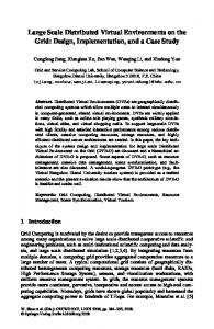
We developed a Ping-Pong game in the Parallel and Distributed Computing Center of the School of Computer Engineering in Nanyang Technological University. The game is played by two players on two PCs running on Windows 2000. The two PCs are connected by a 100Mbps LAN. Figure 5 shows the screen shot of the game.

Fig. 5.

A screen shot of the Ping-Pong game

The game simulates a 30m by 15m court. The ball has a diameter of 0.3m and moves at a constant speed of 6m/s. The initial position of the ball is at the center of the court. When each round of the game starts, the ball moves towards one of the players at a random angle. If the ball hits the sidewall or a bat, we assume the ball’s behavior follows the law of reflection. A player needs to move his/her bat along the baseline to block the ball. We assume that the movement of a bat obeys Newton’s second law of motion. To make the game challenging, the acceleration (a) of a bat is set to 2m/s2 , the maximum speed of a bat is set to 3m/s, and the width of a bat is set to 0.25m. If the ball passes the baseline, then the player at that side loses one point, and the ball is reset to the center of the court for the next round. When one player loses 5 points, then the player loses the game. Message transmission delay ACM Transactions on Computational Logic, Vol. V, No. N, November 2003.

Suiping Zhou et al.

·

11

is introduced to simulate that the game is played by two geographically distributed players. 5.2

Experiment Design

Suppose A and B are the two players playing the game. To capture the different perceptions of the two players, and also to simplify the verification of the proposed metric, we focus on the two players’ perceptions of the bats’ positions. To this end, the ball’s position is kept consistent on the two players’ computer screens, and a first order DR algorithm is used on each player’s computer to estimate the movement of another player’s bat. Thus, when the ball approaches one player, say player A, this player may move his/her bat to block the ball. Suppose the ball is blocked by player A, thus player A will see on his/her screen that the ball is bounced back to player B. However, the inconsistency in the application may cause player B to have a different perception of the position of player A’s bat. Since the ball’s position is always consistent on the two player’s screens, player B may see that the ball is not hit by player A’s bat, however the ball still bounces back. A player is asked to press the space bar whenever he/she observes such abnormal behavior, thus the inconsistent perceptions of the two players are captured. Some important considerations in the experiment design are described as follows. — High resolution clock and clock synchronization - To investigate the effect of network delay and clock asynchrony on the time-space inconsistency of the game, high resolution clocks are used on the two computers. The message transmission delay between these two computers is less than 0.2ms with small variation, thus the two clocks can be considered as perfectly synchronized by using a simple synchronization algorithm. To deal with clock drift, the clock synchronization algorithm is executed at the start of each round of the game. — Consistent position of the ball - At the start of each round, the ball is reset to the center of the court. At time “0”, the ball moves towards one side of the court in a random direction. When the ball is hit by the bat of one player, this information is sent to the other player immediately. Since the transmission delay between the two computers is negligible compared to human perception time, the ball’s position is kept consistent between the two players. — Network delay and clock asynchrony simulation - To simulate the message transmission delay in the Internet, an outgoing message is delayed by some time before it is sent out. The delay is modelled as a random variable x which has an exponential distribution [BERTSEKAS and GALLAGER 1992; CERLLET et al. ; KATO et al. 1999], i.e., fx (t) = λe−λ(t−µ) , t ≥ 0, where fx (·) stands for the probability density function of x. Since the two clocks of the two computers are synchronized with high accuracy, the asynchrony between the two clocks can be easily simulated by adding an offset to one clock. Note that in this game, network delay only has effect on the update messages of the bats, it has no effect on the update messages of the ball, i.e., when the ball is hit by a bat, this message is sent to the other player immediately. — Measurement of ² - To get the value of ² in (3), a series of tests has been ACM Transactions on Computational Logic, Vol. V, No. N, November 2003.

12

·

Time-Space Consistency in Large Scale Distributed Virtual Environments

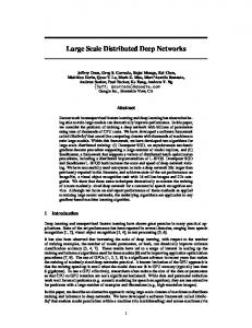
done on three subjects5 . In each test, the ball approaches the bat at the other side of the court. The bat moves at a speed of 0.3m/s. The choice of this speed is based on the observation that in the game, the average speed of a bat when it hits the ball is about 0.3m/s with small variance. When the ball reaches the baseline, the ball is bounced back. Then we ask the subjects to decide whether the bat hit the ball or not. The answer can be “yes”, “no” or “cannot decide”. We controlled the distance between the ball and the bat when the ball reaches the baseline. Five distance groups were used in these tests: (0m, 0.1m), (0.1m, 0.2m), (0.2m, 0.3m), (0.3m, 0.4m) and (0.4m, 0.5m). In each group, 20 distance values were generated randomly. Thus, for each subject, the test was done for 100 times. To decide ², we calculate the frequency that a subject’s answer is “no”, since when the answer is “no”, the subject can clearly discern the gap between the ball and the bat. Figure 6 shows the average frequency of the “no” answers against the different distance groups, where on the horizontal axis, each distance group is represented by its center point. It can be seen from Figure 6 that when the distance between the ball and the bat is 0.1m, the corresponding frequency of the “no” answers is about 0.05, i.e., the probability that a player can discern the gap between the ball and the bat is about 0.05. Thus, we choose ² to be 0.1m in the evaluation of the game.

Fig. 6.

Measurement of ²

— Experiment scenarios and procedure - To “create” different levels of inconsistency, we set different values to some characteristic parameters of the game. The threshold of the DR algorithm (δ) is set to 0.05m, 0.1m and 0.3m respectively. The clock asynchrony (γ) between the two computers is set to 0.01s and 0.2s respectively. We simulate two different network connections between the two computers [CERLLET et al. ; KATO et al. 1999]: 5 Since

the test results on these subjects were close to each other, the test was not done on more subjects. ACM Transactions on Computational Logic, Vol. V, No. N, November 2003.

Suiping Zhou et al.

·

13

(1) Small message transmission delay with small variation: in this case, µ is set to 20ms, λ is set to 1, the corresponding average message transmission delay is Td = µ + 1/λ = 0.021s. (2) Large message transmission delay with large variation: in this case, µ is set to 200ms and λ is set to 0.1, the corresponding value of Td is 0.21s. Six different scenarios were used in the experiment as shown in Table I. These six scenarios were chosen simply because they represent different levels of the parameters, and the corresponding value of ω ranges from 0 to a value much larger than 1. To show how the values in the last column of Table I are calculated, consider test 1 and test 6 as two examples. In test r 1, the average update interval of the DR 2δ ≈ 0.224s. According to (5) and (7), algorithm can be estimated as TDR = |a| we have |∆1 (t)| = 0.3 × 0.01 + 0.05 + 2 × 0.224 × (t − tupdate ) where (t − tupdate ) ∈ [0, 0.021], and |∆2 (t)| = 0.3 × 0.01 + ξ(t) where ξ(t) ∈ [0, 0.05]. Since the maximum value of |∆1 (t)| is less than ², we have Ω1 = 0. For the same reason, we have Ω2 = 0. Thus, we have ω = ² Ω · σ = 0. In test 6, TDR ≈ 0.548s. Thus, we have |∆1 (t)| = 0.3 × 0.01 + 0.3 + 2 × 0.548 × (t − tupdate ) where (t − tupdate ) ∈ [0, 0.21], and |∆2 (t)| = 0.3 × 0.01 + ξ(t) where ξ(t) ∈ [0, 0.3]. According to (6) and (8), we have Ω1 =0.087(m·s), and Ω2 =0.051(m·s). Thus, ω = 9.20. Scenario test 1 test 2 test 3 test 4 test 5 test 6

(δ, Td , γ) (0.05, 0.021, 0.01) (0.10, 0.021, 0.01) (0.05, 0.021, 0.20) (0.10, 0.21, 0.01) (0.30, 0.021, 0.01) (0.30, 0.21, 0.01)

Table I.

ω 0 1.23 1.31 2.67 5.87 9.20

Test scenarios

Five pairs of subjects were formed. Each pair of subjects was tested with these six scenarios. The experiment lasts for 1 to 1.5 hours for each pair. 5.3

Results and Analysis

Before doing experiments with the game, each pair of subjects was given 20 minutes to get familiar with the game. Then, each pair played the game in the six experiment scenarios. The six experiment scenarios were given to each pair in random order. ACM Transactions on Computational Logic, Vol. V, No. N, November 2003.

14

·

Time-Space Consistency in Large Scale Distributed Virtual Environments

Suppose na denotes the total number of instances of abnormal behavior that a pair of subjects observed when playing the game in an experiment scenario, and nb denotes the total number of times that the ball was hit back in the same scenario. Since each game may last for different periods depending on the players’ skills, we a use n nb as an index of the frequency that abnormal behavior is observed in the game. Experimental results are shown in Table II. In Figure 7, the average value a of n nb is drawn against the value of ω in different scenarios. na /nb group1 group2 group3 group4 group5 Average

test 1 0.022 0.025 0.012 0.011 0.059 0.026

test 2 0.11 0.085 0.074 0.099 0.115 0.097 Table II.

Fig. 7.

test 3 0.142 0.227 0.140 0.152 0.094 0.151

test 4 0.271 0.212 0.216 0.231 0.170 0.220

test 5 0.305 0.278 0.250 0.276 0.229 0.268

test 6 0.305 0.461 0.459 0.386 0.356 0.393

Test results

a Average value of n nb

As can be seen from Figure 7, with the increase of ω, the subjects will observe a abnormal behavior more frequently. n nb is small (< 0.08) when ω < 1, but increases very fast when ω is around 1. The results show that the game has a good time-space consistency property when ω < 1, and the larger the value of ω, the worse the timespace consistency property of the game. The results also clearly show the effect of various parameters on the performance of the game. For example, in test 1, test 2 and test 5, with the increase of δ, ω also increases, and the performance of the a game is degraded - n nb increases from 0.026 in test 1 to 0.268 in test 5. The impact of network latency on the performance of the game is obvious. For example, in test 2 and test 4, with the increase of Td from 0.021s to 0.21s, ω increases from 1.23 to a 2.67, and n nb increases from 0.097 to 0.22. To see the effect of clock asynchrony, ACM Transactions on Computational Logic, Vol. V, No. N, November 2003.

Suiping Zhou et al.

·

15

γ is increased from 0.01s in test 1 to 0.2s in test 3. The corresponding value of ω a increases from 0 to 1.31, and n nb increases from 0.026 to 0.151. 6.

RELATED WORK

Maintaining a consistent view of the simulated world among different simulation nodes is a fundamental problem in DVEs. There are many issues concerning this fundamental problem, and a lot of related work has been done in recent years [ALEX and TAYLOR 2000; CAI et al. 1999; ROBERTS and SHARKEY 1997; DIOT and GAUTIER 1999; KOH et al. 2000; LUI et al. 1999; MORSE et al. 2000]. In [DIOT and GAUTIER 1999], Diot and Gautier use “drift distance” to evaluate the inconsistency in a distributed game. The drift distance represents, in distance units, the absolute value of the distance between the position of an avatar as displayed by its local entity, and the position of the same avatar as displayed by a remote entity. The game is called inconsistent if the drift distance is large compared to the avatar’s size. This metric does not consider the effect of the duration of the situation caused by the distance drift. As the authors noticed in [DIOT and GAUTIER 1999]: A small error on the position of a very slow avatar can be dramatic, while the same error on a very fast avatar would not be visible to the players (if the error is along the trajectory of the avatar). The reason for this is that it takes a shorter time for a fast avatar to cover the same drift distance than for a slow avatar, i.e., the situation caused by the same drift distance will last for a shorter time for a fast avatar than for a slow avatar. In [LUI et al. 1999], the authors use “phase difference” to evaluate the inconsistency in a DVE. For example, suppose client A starts to render an entity’s state at time step i, and client B starts to render the same state of that entity at time step j (> i), then the phase difference between client A and client B is defined as j − i. Phase difference only considers how long a situation lasts, it does not consider the position difference caused by the phase difference. In fact, for a fast entity, the position difference caused by the same phase difference can be quite different from that for a slow entity. The time-space inconsistency defined in this paper combines the effect of position difference and the effect of its duration. We believe that both the position difference and the duration of the situation caused by the difference have great impact on participants’ judgements and actions in a DVE application. Our work clearly shows how the characteristic parameters of a DVE are interrelated to each other in deciding the time-space inconsistency in the application. For example, as can be seen from (6) and (8), the impact of clock asynchrony on a fast moving entity is more significant than on a slow entity. With the increase of δ, TDR also increases, the impact of clock asynchrony and network latency both increases, thus the accuracy of the DR algorithm is very important for DVEs. Furthermore, with the increase of the maximum acceleration of an entity, the impact of network latency increases very fast. Thus for DVE applications with highly agile entities such as fighter jets, the network latency needs to be kept as small as possible. In general, to reduce the time-space inconsistency in a DVE application, we need to reduce the message transmission delay, use high accuracy clocks and synchronization schemes, and use accurate DR algorithms. We do not ACM Transactions on Computational Logic, Vol. V, No. N, November 2003.

16

·

Time-Space Consistency in Large Scale Distributed Virtual Environments

elaborate on these issues in this paper, interested readers may refer to [ALEX and TAYLOR 2000; CAI et al. 1999; ROBERTS and SHARKEY 1997; DIOT and GAUTIER 1999; KOH et al. 2000; LUI et al. 1999; MILLS 1992; MORSE et al. 2000]. 7.

CONCLUSIONS

In this paper, we investigate the time-space consistency problem in large scale DVEs. A metric is defined to characterize the time-space inconsistency in a DVE application. Our work clearly shows how time-space inconsistency is decided by the characteristic parameters of a DVE application. Thus, the time-space consistency property of a DVE application can be evaluated without the actual execution of the DVE application, which is especially useful in the design stage of a new DVE. To verify the proposed metric, a Ping-Pong game is developed. Experimental results with the game show that the metric is effective in evaluating the time-space consistency property of the game. Our work also provide some guidelines on how to fine-tune the parameters of a DVE to reduce the time-space inconsistency. Generally, from the system point of view, high speed networks and fast message transmission protocols should be used to reduce the message transmission delays, and high accuracy clocks and synchronization schemes should be used to minimize the clock asynchrony. From the application point of view, accurate DR algorithms should be used, but this will result in extra overheads in the communication networks and simulation nodes. To make a good trade-off, we need to quantify the time-space inconsistency and know how it is affected by the parameters of a DVE. In this paper, we answer this question by showing how the characteristic parameters of a DVE are interrelated to each other in deciding the time-space inconsistency, so that we may fine-tune the DVE to make it as consistent as possible. ACKNOWLEDGMENTS

We would like to thank the anonymous referees for their very valuable comments and insightful suggestions which helped improve the quality and presentation of this paper. We are also grateful to Mr. Hanfeng Zhao for his help in setting up the game and the experiments. REFERENCES ALEX, K. and TAYLOR, S. 2000. Using determinism to improve the accuracy of dead reckoning algorithms. In Proceedings of the Simulation Technology and Training Conference. Sydney, Australia. ANDERSON, D. B. et al. 1995. Building multi-user interactive multimedia environments at MERL. IEEE Multimedia 2, 4, 77–82. BERTSEKAS, D. and GALLAGER, R. 1992. Data Networks. Prentice Hall, New Jersey. CAI, W., LEE, B., and CHEN, L. 1999. An auto-adaptive dead reckoning algorithm for distributed interactive simulation. In Proceedings of the Thirteenth Workshop on Parallel and Distributed Simulation. Atlanta, GA, USA, 82–89. CARLETON, L. 1981. Processing visual feedback for movement control. Journal of Experimental Psychology: Human Perception and Performance 7, 5, 1019–1030. CERLLET, A., PULLIN, D., and SARGOOD, S. Statistics of one-way Internet packet ACM Transactions on Computational Logic, Vol. V, No. N, November 2003.

Suiping Zhou et al.

·

17

delays. Available from http://www.globecom.net/ietf/draft/draft-corlett-statistics-of-packetdelays-00.html. DEERING, M. 1992. High resolution virtual reality. Computer Graphics 26, 2 (July), 195–201. DIOT, C. and GAUTIER, L. 1999. A distributed architecture for multiplayer interactive applications on the Internet. IEEE Network 13, 4, 6–15. FUJIMOTO, R. M. 1998. Time management in the high level architecture. Simulation 71, 6 (Dec.), 388–400. FUJIMOTO, R. M. 1999. Parallel and distributed simulation. In Proceedings of the 1999 Winter Simulation Conference. Phoenix, Arizona, USA, 122–131. HAGSAND, O. 1996. Interactive multiuser VEs in the DIVE system. IEEE Multimedia 3, 1, 30–39. IEEE. 1993. Standard for distributed interactive simulation. IEEE Std.1278 . IEEE. 2000. The high level architecture. IEEE Std.1516 . KATO, J.-Y., SHIMIZU, A., and GOTO, S. 1999. Active measurement and analysis of delay time in the Internet. In Proceedings of the 1999 International Workshops on Parallel Processing. Wakamatsu, Japan, 21–24. KOH, J. et al. 2000. Multi-cast fast messages in RTI-kit. In Proceedings of the 2000 Spring Simulation Inter-operability Workshop. Orlando, Florida, USA. LUI, C., SO, K., and TAM, T. 1999. Deriving communication sub-graph and optimal synchronizing interval for a distributed virtual environment system. In Proceedings of the IEEE International Conference on Multimedia Computing and Systems. Florence, Italy, 357–361. MILLER, D. C. and THORPE, J. A. 1995. SIMNET: the advent of simulator networking. Proceedings of the IEEE 83, 8 (Aug.), 1114–1123. MILLS, D. 1992. Network time protocol (version 3) specification, implementation and analysis, RFC-1305. MORSE, K., BIC, L., and EILLENCOURT, M. 2000. Interest management in large scale virtual environments. Presence 9, 1 (Feb.). ROBERTS, D. and SHARKEY, P. 1997. Maximising concurrency and scalability in a consistent, causal, distributed virtual reality system whilst minimizing the effect of network delays. In Proceedings of the 6th Workshop on Enabling Technologies Infrastructure for Collaborative Enterprises. MIT, Cambridge, MA, USA, 161–166. SINGHAL, S. and ZYDA, M. 1999. Networked Virtual Environments: Design and Implementation. Addison-Wesley. WARE, C. and BALAKRISHNAN, R. 1994. Reaching for objects in vr displays: lag and frame rate. ACM Transactions on Computer-Human Interaction 1, 4, 331–356.

Received Month Year; revised Month Year; accepted Month Year

ACM Transactions on Computational Logic, Vol. V, No. N, November 2003.