Time synchronization errors in GPS-aided inertial

IEEE TRANSACTIONS ON INTELLIGENT TRANSPORTATION SYSTEMS, VOL. X, NO. X, XXXX 200X

1

Time synchronization errors in GPS-aided inertial navigation systems Isaac Skog and Peter H¨andel

Abstract—The effects of time synchronization errors in a GPSaided inertial navigation system (INS) are studied in terms of the increased error covariance of the state vector. Expressions for evaluating the error covariance of the navigation state vector— given the vehicle trajectory and the model of the INS error dynamics—are derived. Two different cases are studied in some detail. The first case considers a navigation system in which the timing error is not included in the integration filter. This leads to a system with an increased error covariance and a bias in the estimated forward acceleration. In the second case, a parameterization of the timing error is included as a part of the estimation problem in the data integration. The estimated timing error is fed back to control an adjustable fractional delay filter, synchronizing the inertial measurement unit (IMU) and GPS-receiver data. Simulation results show that by including the timing error in the estimation problem, almost perfect time synchronization is obtained and the bias in the forward acceleration is removed. The potential of the proposed method is illustrated with tests on real-world data that are subjected to timing errors. Moreover, through an observability analysis, it is shown that the timing error is observable for all trajectories that include turns or non-zero accelerations. Index Terms—Time synchronization, vehicle navigation, global positioning system (GPS), inertial navigation system (INS)

Nomenclature Subscripts and superscripts (·)n Quantity in navigation coordinates. (·)p Quantity in platform coordinates. (·)f Quantity in the system with feedback. (·)ext Quantity in the system with a state model extended to also include the time synchronization error. (·)f d Quantity in the feedback system with time delay. (·)c Continuous time variable (·)k Time index, discrete time. [·]i:j Element i to j in a vector. (·)T Transpose operator. (·)a Actual value. Predicted value. (·)− k ˜· Measured value. b· Estimated value. · Average value. Scalars α Length of the state vector z. β Length of the position vector p. φ Tilt (pitch) angle.

Manuscript received I. Skog and P. H¨andel are with the ACCESS Linnaeus Center, KTH Signal Processing Lab, Royal Institute of Technology.

M Ts Td δTd D 2 2 2 , σgps , σgyro σacc

Vectors x

δx u

δu z = [δxT δuT ]T d e w r θ p(t), pk v(t), vk a(t), ak s(t), sk ω(t), ωk Matrices Ij 0i,j (0i )

Ratio between the sampling rate of the IMU and the GPS-receiver. Sampling period of the IMU. Time synchronization error. Perturbation in the estimate of the time synchronization error (i.e., δTd = Tda − Tbd ). Normalized time synchronization error Variance of the accelerometer, gyro, and GPS measurement noise, respectively. State vector, containing the position, velocity, and attitude of the navigation system. Perturbation in the state vector (i.e., b). δx = xa − x Input vector, containing the accelerations and angular rates of the navigation platform. Perturbation in the estimated sensor errors (i.e., δu = δua − δb u). Extended state vector. Bias vector due to the time synchronization error. IMU measurement noise. GPS measurement noise. Difference between the position estimated by the GPS and INS. Vector of Euler angles. Position vector in continuous and discrete time, respectively. Velocity vector in continuous and discrete time, respectively. Acceleration vector in continuous and discrete time, respectively. Specific-force vector in continuous and discrete time, respectively. Angular-rate vector in continuous and discrete time, respectively. Identity matrix of size j. Zero matrix of size i × j (i × i).

PSfrag replacements

IEEE TRANSACTIONS ON INTELLIGENT TRANSPORTATION SYSTEMS, VOL. X, NO. X, XXXX 200X t = k Ts

IMU

frag replacements

bk ) bk+1 = f (b xk − δb xk , u x

accelerometers gyros

Navigation t = l T s − Td , l = k M

Filter

IMU

Sensor error compensation

δb uk

Position Velocity Attitude

˜k u

2

bk u

Navigation Equations

bk+1 x

δb xk

− Kk

GPS

+

Hk

+

GPS

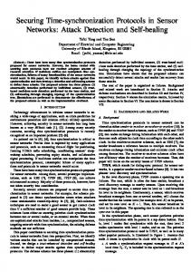
Fig. 1. Effects of the timing error Td in the synchronization between the sampling of the GPS-receiver and IMU are studied in terms of the navigation system’s increased error covariance. Here, the ratio between the sampling rate of the IMU and GPS-receiver is assumed to be an integer m ≥ 1.

Kalman prediction gain matrix. Kalman filter gain matrix. State transition matrix Observation matrix. Process noise matrix. Covariance matrix. Process noise covariance matrix Observation noise covariance matrix. Observability matrix.

Kp K Ψ H G P Q R Wo Functions x˙ c = fc (xc , uc ) xk+1 = f (xk , uk ) δi,j E{·} S(a) ∆(k)

Continuous time navigation equations. Discrete time navigation equations. Kronecker delta function. Expectation operator. Skew symmetric matrix representation of the vector a. That is a × b = S(a) b. Downsampling function.

I. INTRODUCTION One of the first problems encountered when investigating the practical construction of low-cost GPS-aided inertial navigation systems (INS) based on commercial off-the-shelf components (COTS) is the problem of time synchronization in the sampling of the GPS-receiver and inertial measurement unit (IMU). Since in most cases there is no direct access to the hardware of the sensor modules and no possibility of modifying their internal software, the data synchronization between GPS and IMU must be done in an ad-hoc manner. Therefore, one often encounters a small timing error between the sampling instances of the GPS-receiver and the IMU. The setup considered is illustrated in Fig. 1. The timing error gives rise to several questions: what is the impact on the accuracy of the navigation system? how large can the errors be for a given accuracy? and how to estimate and compensate for it? The impact of data timing errors in integrated navigation systems was first studied in [1], where it was shown that the data timing errors may cause a bias in the forward acceleration during the transfer alignment of a strap-down INS. In [2], [3] and [4], the effects of using time-delayed GPS measurements in a GPS-aided strap-down INS were studied by examining the steady-state condition of the Kalman filter that was used to fuse navigation data. Further, in [2], a calibration procedure

b INS p k+1

b GPS p k+1

Fig. 2. Block diagram of a closed-loop GPS-aided INS model. The EKF recursions used to fuse the GPS-receiver and the IMU data may be interpreted as a way of choosing the gain matrices Kk in the feedback.

was proposed based on driving the vehicle with the GPSaided INS according to a predefined trajectory. A few methods for synchronizing the data streams at the hardware level are described in [5], [6] and [7]. In this paper, the impact of a time synchronization error in a closed-loop GPS-aided INS is studied in terms of the increased error covariance of the system. In Section II, by modeling the timing error as a trajectory-dependent bias in the GPSreceivers position estimates and by studying the behavior of navigation errors in the closed-loop GPS-aided INS, a stochastic difference equation for the navigation errors in the system with timing error is found. From this equation, an expression for the error covariance of the closed-loop system with timing error is derived. In Section III, the case when the timing error is included in the estimation problem is studied. By including the timing error in the feedback loop of the navigation filter, almost perfect time synchronization is achieved. The general theoretical findings in Section II and III are illustrated by an example of a single-axis GPS-aided INS in Sections II-C and III-A, respectively. In Section IV, a practical approach to the implementation of the time synchronization, using an adjustable fractional delay filter to delay the IMU data, is described. The proposed time synchronization approach, using a fractional delay filter, is included as a part of the inhouse developed software for simulations and tests for lowcost GPS-aided INSs. In Section V, the integration software and the time synchronization are tested with both simulated and real-world data, subjected to synchronization errors. In Section VI, the observability of the timing error is examined. Finally, in Section VII, conclusions are drawn and the results summarized. II. C OVARIANCE OF THE ESTIMATION ERROR To evaluate the effects of the time synchronization error on the performance of the navigation system, the method that is used to fuse the sensor data must be specified. In this paper, a feedback implementation of a complementary filter is used to fuse the navigation data. That is, given a linear state space model of how the position, velocity, attitude, and sensor errors in the mechanization of the INS develop with time, a standard Kalman filter is used to estimate the error state of the INS. The estimated navigation errors are then fed back into the INS to correct its internal states. Since the model for the error plant of the INS depends on the current navigation state, an indirect extended Kalman filter is created. Hence, to

IEEE TRANSACTIONS ON INTELLIGENT TRANSPORTATION SYSTEMS, VOL. X, NO. X, XXXX 200X

evaluate how the timing error will affect the performance of the navigation system, the state-space model of the error plant and the extended Kalman filter recursions must be studied. Introduce a state vector zk of the form   δxk zk = (1) δuk

where δx contains the position, velocity, attitude perturbation of the INS, and δuk the IMU sensor errors. Then the error plant of the INS can be described by a state-space model of the form

TABLE I T HE INDIRECT EXTENDED K ALMAN FILTER ALGORITHM FOR INTEGRATION BETWEEN GPS- RECEIVER AND IMU DATA , WITH A RATIO BETWEEN THE SAMPLE RATES EQUAL TO M TIMES . No GPS data available. (k 6= n M , n = 1, 2, ...) ˜ k + δ u− u− k =u k − − xk+1 = fd (x− k , uk ) − δ u− k+1 = δ uk − T T P− k+1 = Ψk Pk Ψk + Gk Q Gk

GPS data available. (k = n M , n = 1, 2, ...) − T T −1 Kk = P − k Hk (Hk Pk Hk + Rk )


zk+1 = Ψk zk + Gk ek

(2)







0α×1 δ xk x− k = + Kk (pGPS − Hk ) k δ uk δ u− 0 β×1 k 

where the state transition matrix Ψk describes how the errors develop from one time instance to another and can be found by a perturbation analysis or linearization of the mechanized navigation equations and sensor models. Refer to the standard text-books [8], [9], [10], or [11] for more details on how this is done. Further, the process noise gain matrix Gk describes how the measurement noise ek from the inertial sensors affects the navigation error. Since the GPS and IMU in most cases are sampled at two different rates, introduce the following downsampling function  1, k = nM, n = 1, 2, ... ∆(k) = . (3) 0, otherwise

Here, M denotes the ratio between the sampling rate of the IMU and the GPS-receiver, and is taken to be an integer. If the difference between the position estimates of the GPS and the INS is observed, the observation equation for the state-space model is given by rk = Hk zk + ∆(k)wk

(4)

where the observation matrix Hk is defined as Hk = ∆(k)[Iβ 0β,(α−β) ].

(5)

The integers α and β denote the length of the state vector zk and position vector rk , respectively. The notations Iβ and 0β,(β−α) denote a unity matrix of size β and a β × (β − α) matrix with zeros, respectively. The GPS-receiver positioning error1 wk and the measurement noise ek of the inertial sensors are considered as white noises, uncorrelated with each other and with covariance matrices R = E[wk wkT ]

Q = E[ek eTk ].

(7)

For an error model of the form (2)–(7) the corresponding extended Kalman filter recursions, used to fuse the IMU and GPS-receiver data in a closed-loop system, are given in Table I, 1 In

reality, the errors in the positioning estimates of the GPS-receiver are correlated both in time and space with a covariance structure depending on the positioning algorithm of the GPS-receiver [8].





e xk = x− k + xk ˜ k + δ uk uk = u Pk = (I − Kk Hk ) P− k x− k+1 = fd (xk , xk )

δ u− k+1 = δ uk T T P− k+1 = Ψk Pk Ψk + Gk Q Gk

as derived in [12]. This set of equations may graphically be interpreted as the closed-loop system in Fig. 2, where the feedback gain is chosen as the Kalman filter gain. A. Closed-Loop Error To find a difference equation for the error in the closedloop system described by the indirect extended Kalman filter algorithm in Table I, it should be noted that when GPS data is available, the current error state is estimated as b zk = K k rk .

(8)

That is, the current perturbation in position, velocity, and attitude δxk and the current error in the estimated sensor perturbation δb uk are equal to the position error times the Kalman filter gain. This error estimate is used to correct the current navigation state of the INS before the time update. Thus, the state error after the feedback is the error before feedback zf,k minus the estimated error b zk . With reference to (2), describing how the state errors relate from one time instance to the next, the error of the closed-loop system zf,k is found to be zf,k+1

(6)

and

3

= =

Ψk (zf,k − b zk ) + G k e k

Ψk zf,k − Ψk Kk rk + Gk ek .

(9)

Equation (9) can be written in a more convenient form by using the definition of the observation vector rk in (4) and by noting that Kp,k = Ψk Kk is the one-step-ahead Kalman prediction gain. Thus (9) may be rewritten as zf,k+1

=

Ψk zf,k − Kp,k (Hk zf,k + ∆(k) wk ) + Gk ek

=

(Ψk − Kp,k Hk ) zf,k − Kp,k wk + Gk ek . (10)

In the second equality, one used that the Kalman gain Kk per definition, and hence the prediction gain Kp,k are zero

IEEE TRANSACTIONS ON INTELLIGENT TRANSPORTATION SYSTEMS, VOL. X, NO. X, XXXX 200X

matrices, whenever the downsampling function ∆(k) in (3) is zero. Equation (10) can be identified as the difference equation describing the error of the one-step-ahead Kalman filter predictor. Indeed, it is shown in [13] that for a linear system, the optimal choice of the feedback gain is the Kalman predictor gain, resulting in a system with an error covariance equal to that of the linear Kalman predictor. Thus, the error covariance of the system with feedback is given by the onestep-ahead Kalman predictor error covariance. In summary, the stochastic difference equation (10) describes how the errors in the estimated position, velocity, attitude, and sensor errors propagate with time in the closedloop implementation of a GPS-aided INS. The dynamics of the errors in the system are determined by the time varying closed-loop system matrix (Ψk −Kp,k Hk ), which depends on the trajectory dynamics of the navigation platform. Therefore, analytical results about the convergence of the errors in the navigation system are difficult to present. Further, the error covariance of the closed-loop system is given by the one-stepahead Kalman predictor covariance and not, as first may be expected, the Kalman filter covariance. This occurs because the system cannot instantaneously respond to the feedback control [13]. B. Timing Errors in Closed-Loop Now consider the case when there is a timing error between the sampling of the GPS-receiver and the IMU, so that their sampling instants are not perfectly aligned (see Fig. 1). Let this constant misalignment in the sampling instant be denoted Td and assume that it occurs in the sampling of the GPS-receiver. Further, let the function p(t) describe the true trajectory of the navigation platform. Then the position estimates from the GPS-receiver at time k can be described as b GPS = ∆(k)(p(k Ts − Td ) + wk ) p k

(11)

where wk is the estimation error of the GPS-receiver. Assume that a rough synchronization of the GPS-receiver and IMU data has been done by means of correlation or at hardware-level, so that |Td | is in the order of a few sampling periods Ts . Then p(k Ts − Td ) in (11) can be approximated by a second-order Taylor expansion around t = k Ts , that is, T2 (12) p(k Ts − Td ) ' pk − vk Td + ak d 2 where pk , vk , and ak denote the navigation platform position, velocity, and acceleration at sampling instance k, respectively. The symbol ' denotes equality where only the significant terms have been retained. Inserting (12) into (11) gives b GPS p k



Td2



(13) + wk . 2 Thus, the true observation rak of the system, which is fed back into the closed-loop system, can be described as rak

' ∆(k) pk − vk Td + ak

= '

b INS −p ∆(k)(b pGPS k ) k

∆(k)(pk − vk Td + ak

Td2 b INS + wk − p k ). (14) 2

4

b INS is the position estimate from the INS at time Here p k b INS k. Next, identifying that Hk zek = ∆(k)(pk − p k ) and substituting it into (14) yields the following description of the true observation for the system with a timing error rak ' ∆(k)(Hk zk + wk + dk ).

(15)

In (15), the position error vector dk is introduced as Td2 . (16) 2 By comparing (15) and (4) it is clear that the actual observation contains not only the position error and measurement noise but also a bias term dk that depends on the timing error Td and the dynamics of the navigation system. Substituting rk with rak in (9) and inserting (15) into this yields the following difference equation for the error state in the closedloop navigation system with timing errors dk = −vk Td + ak

zf d,k+1

Ψk zf d,k − Kp,k rak + Gk ek   Ψk zf d,k − Kp,k ∆(k)(Hk zk + wk + dk )

= = +

(17)

G k ek .

By examining the recursions in Table I it is clear that the Kalman filter gain Kk and hence also the Kalman filter prediction gain Kp,k are zero whenever ∆(k) is zero. Thus (17) can be rewritten into a more familiar form = −

zf d,k+1

(Ψk − Kp,k Hk ) zf d,k − Kp,k wk + Gk ek Kp,k dk . (18)

Equation (18) has similarities with the difference equation (10) describing the estimation error in the closed-loop system without timing error except from the last additional term Kp,k dk reflecting the contribution due to timing error. Next, introduce Φk =



Ψk − Kp,k Hk , Ψk ,

k = n M, n = 1, 2, ... otherwise

(19)

Then the covariance of the estimation error may be expressed as Pf d,k+1

= = +

E[zf d,k+1 (zf d,k+1 )T ] Φk Pf d,k ΦTk + Kp,k R LTk + Gk Q GTk Kp,k dk dTk LTk − Φk E[zf,k ] dTk LTk

−

Kp,k dk E[zf,k ]T ΦTk

(20)

where the mean of the estimation error can be calculated as E[zf,k+1 ] = Φk E[zf,k ] − Kp,k dk .

(21)

The derived expressions (20) and (21) describe the dynamics of the covariance and mean of the navigation errors in a closedloop GPS-aided integrated navigation system with timing error. The three last terms in equation (20) are the contribution to the covariance due to time delay, whereas the three former

IEEE TRANSACTIONS ON INTELLIGENT TRANSPORTATION SYSTEMS, VOL. X, NO. X, XXXX 200X

5

satellite

satellite

xc = and input vector



p(t)

uc = accelerometer sensitivity axis

ω ˜ (t)

gravity vector

s(t)

φ(t)

ω(t)

T

T

acceleration a ˜(t)

(26)

(27)

x˙ c = fc (xc , uc )

gravity vector

Fig. 3. Example of a single-axis GPS-aided INS system. The acceleration and tilt rate of the vehicle are measured by an accelerometer and a gyro mounted at the center of gravity of the vehicle. When the vehicle accelerates it tilts and the accelerometer will not only sense the forward acceleration but also the gravity force. The position of the vehicle is estimated using a GPS-receiver having an inherent time delay.

ones correspond to the case when there is no time delay. As for the case without timing error, the error dynamics are determined by the time-varying system matrix Φk and now also the position bias dk , both depending on the trajectory of the navigation platform. Therefore, general analytical results of the convergence of the estimation errors are difficult to derive. However, the derived expressions can be numerically evaluated to investigate how the sampling timing error will affect the accuracy of the navigation system for a certain trajectory.

Assuming that there is a bias δω and noise ec,2 in the gyro measurements, whereas the accelerometer measurements are only disturbed by some noise ec,1 2 , the measured output from the accelerometer and gyro can be described as

Consider the single-axis navigation problem illustrated in Fig. 3 with reference to, for example, performance measurements in drag racing type of activities [14]. The purpose is to determine the position of the vehicle along a horizontal straight track. The vehicle is equipped with a GPS-receiver that gives noisy position estimates at 10 Hz. The acceleration and tilt rate of the vehicle are measured by an accelerometer and a gyro mounted at the center of gravity of the vehicle. When the vehicle accelerates it will start to tilt and the accelerometer will not only sense the forward acceleration but also the gravity retardation force. Assume the gravity vector to have the magnitude g, the relationship between the acceleration and angular rate of the vehicle and its tilt angle, velocity, and position can be described by the following set of differential equations: (22) (23) (24)

Here p(t), v(t), s(t), φ(t), and ω(t) denote the position, velocity, specific force, tilt, and angular rate of the vehicle, respectively. These equations are referred to as the navigation equations used in the INS to calculate the position, velocity, and tilt from the measured accelerations and angular rates. By introducing the state vector

s˜c = sc + ec,1

(28)

ω ˜ c = ωc − δ ω + ec,2

(29)

and respectively. Using these measurements as the input to the INS results in an error in the calculated position, velocity, and tilt. A linear model for how the errors develops with time may be found by linearizing the navigation equations around the true trajectory, that is, b˙ c x

= =

x˙ ac − δ x˙ c ˜ c) fc (b xc , u

'

fc (xac , uac )

C. Example: Single-axis GPS-aided INS

p(t) ˙ = v(t) v(t) ˙ = s(t) cos−1 (φ(t)) − g tan(φ(t)) ˙ φ(t) = ω(t)

(25)

the continuous time navigation equations (22)–(24) may be written as

PSfrag replacements

b INS p k+1 b GPS p k+1



v(t)

−

∂fc (x, u) ∂fc (x, u) − δxc + ec,1 ∂x x=xa ∂s u=ua

c ∂fc (x, u) (δω − ec,2 ). ∂ω u=ua

c

(30)

c

Hence, assuming that the bias δω in the angular rate measurements is constant, then the errors in the single-axis INS can be modeled as   δ x˙ c (31) = Ψc zec + Gc ec z˙ c = δ ω˙ where

ec = 

and

0  0 Ψc =   0 0 



1 0 0 0

ec,1

ec,2 0

T

sc sin(φc )−g cos2 (φc )

0 0

(32)  0 0   1  0

 0  cos−1 (φc ) 0  . Gc =   0 1  0 0

(33)

0

(34)

2 Including a bias term in the description of the accelerometer measurement would result in a nonobservable state-space model of how the single-axis INS errors develops with time.

IEEE TRANSACTIONS ON INTELLIGENT TRANSPORTATION SYSTEMS, VOL. X, NO. X, XXXX 200X

[m]

TABLE II S ETTING USED WHEN EVALUATING THE SINGLE - AXIS GPS- AIDED INS WITH THE AID OF NUMERICAL SIMULATIONS .

Position

4000 2000 0

0

20

40

[m/s]

80

100

60

80

100

Value

Parameter

Value

σgps σacc σgyro Td ? Tmax ? Tmin Ts

0.5 [m] 0.01 [m/s2 ] 0.1 [◦ /s] 0.1 [s] 0.1 [s] 0 [s] 10 [ms]

[Pf d,0 ]1,1 [Pf d,0 ]2,2 [Pf d,0 ]3,3 [Pf d,0 ]4,4 [Pf d,0 ]5,5 ? [zef d,0 ]6 ? M

0.12 [m2 ] 0.12 [(m/s)2 ] 22 [(◦ )2 ] 0.12 [(◦ /s)2 ] 1/300 [s2 ] 0.05[s] 10

20 0

0

20

40

Tilt

10 [ ◦]

PSfrag replacements

60

Parameter Velocity

40

Notes: The covariance matrix Pf d,0 was initialized as a diagonal matrix with diagonal elements as given in the table. The initial mean error zef d,0 was set to zero, except from the timing error that was set according to the table. This corresponds to initializing the timing error as zero in the navigation filter. Note that the variables denoted with ? and  only exist when the timing error is and is not included in the feedback of the GPS-aided INS, respectively. All other variables are the same for both cases.

0 −10

0

20

40

Time [s]

60

80

100

Fig. 4. Trajectory used in the single-axis GPS-aided INS example. The vehicle tilt is modeled as the output of a first-order system driven by the forward acceleration. [m]

where = I5 + Ts Ψc (k Ts )  1 Ts 0 0  0 1 Ts sc (k Ts )2sin(φc (k Ts ))−g 0 cos (φc (k Ts )) =   0 0 1 Ts 0 0 0 1   0 0  Ts cos−1 (φc (k Ts )) 0   Gk = Gc (k Ts ) =   0 1  0 0   2 σacc 0 δk,l Qk,l = E[ek (el )T ] = 2 0 σgyro



 (36)  (37)

(38)

Further, since the difference in the estimated position of the GPS-receiver and the INS is observed, the observation equation for the error model becomes rk = H k zk + w k

(39)

where =

Qk,l

=



[1 01,4 ] 01,5

, k = nm, n = 1, 2, ... , otherwise

2 E[wk wlT ] = σGP S δk,l .

(40) (41)

10

20

30

40

50

60

70

80

90

100

80

90

100

80

90

100

Standard deviation of the velocity estimation error

0.5 0

0

10

20

30

40

50

60

70

Standard deviation of the tilt estimation error

3 2 1 0

Ψk

0

1

PSfrag replacements

(35)

2 0

[ ◦]

zk+1 = Ψk zk + Gk ek

Standard deviation of the position estimation error

4

[m/s]

In the error model (31)–(34), both the state transition matrices Ψc and Gc are time varying since they depend on the specific force sc and the tilt angle φc . If the sample rate of the INS is high compared to the rate of change in Ψc and Gc , then a zero-order hold sampling of the system results in the following discrete time model for the error in the navigation system.

Hk

6

0

10

20

30

40

50 [s]

60

70

Fig. 5. Standard deviation of the estimation error in the position, velocity, and tilt for a time synchronization error of 100 [ms]. (a) No timing error – red line, (b) Theoretical – black line, (c) Empirical – blue line.

Recall that m is the ratio between the sampling ratio of the IMU and the GPS-receiver. Having derived the state-space model for the error plant in the single axis INS system, which has the same structure as the error model in (2)–(7), the results in (20)–(21) can be applied to evaluate how the time delayed GPS measurements will affect the accuracy of the integrated navigation system given a certain vehicle trajectory. Consider, for example, the vehicle trajectory described in Fig. 4, then the expected performance in terms of the root mean square (rms) and mean error in the integrated navigation system for a time synchronization error of 100 ms is shown in Figs. 5–6. In the example, the system parameters are those given in Table II. A Monte Carlo simulation of the single-axis navigation example was also conducted to illustrate the error model in (20)–(21). The empirical estimated error covariances and means are indicated in black in Figs. 5–6 and show good agreement with those estimated by the error model.

IEEE TRANSACTIONS ON INTELLIGENT TRANSPORTATION SYSTEMS, VOL. X, NO. X, XXXX 200X

b INS where p d,k is the INS position estimates at time instant k calculated from IMU data that has been delayed by Tbd,k seconds. By following the same procedure as in (11)–(14), but expanding the Taylor series around k Ts − Tbd,k instead, it can be shown show that the true observation in the extended state space-model can be expressed as

Standard deviation of the gyro bias estimation error

0.2

[◦ /s]

0.15 0.1 0.05 0

0

20

40

60

80

100

Mean of the gyro bias estimation error

0.15

2  δTd,k e ∆(k) pd,k − vd,k δTd,k + ad,k 2  INS + wk − pd,k .

ra,ext k

=

[◦ /s]

0.1

PSfrag replacements ◦

[ /s]

0.05

0

20

40

60

80

100

[s]

Fig. 6. Standard deviation and mean of the error in the gyro bias estimates for a time synchronization error of 100 [ms]. (a) No timing error – red line, (b) Theoretical– black line, (c) Empirical – black line.

ext ext ra,ext = ∆(k) (Hext k zk + w k + d k ) k

where Hext k = and

III. M ODELLING THE TIMING ERROR IN THE INTEGRATION FILTER

Assume that the integrated navigation system has been extended to also estimate the timing error Td , which then is fed back and used to adjust the sampling instants of the IMU to synchronize it with the sampling of the GPS-receiver. Alternatively, assume that the estimated timing error Tbd (where the b denotes an estimated quantity) is fed back to control a fractional delay filter synchronizing the GPS-receiver and IMU data streams (Fig. 7). Then the plants of the errors in the integrated navigation system can be described by extending the state vector and error model in equations (2)–(6) as follows zext k+1

(42)

ext ext Ψext k zk + G k e k

=

where zext is the augmented state vector (43)

T T zext k = [zk δ Td,k ] .

Further, Ψext k Gext k



=



=

Ψk 01,α Gk 0

0α,1 1 



(44)

Here δTd,k denotes the error in the estimated time delay at time instant k, that is δTd,k = Tda − Tbd,k . The true observation can then be described as ra,ext k

b INS p d,k )

=

∆(k)(b pGPS k

=

+ wk − (46) ∆(k) p(k Ts −   b INS ∆(k) p(k Ts − Tbd,k − δTd,k ) + wk − p d,k

=



−

Tda )

b INS p d,k





Hk

−vd,k

(48)



(49)

2 δTd,k . (50) 2 Hence, the bias in the position error that is fed back into the system with the extended error model is only a function of the accelerations of the vehicle and the timing error δTd,k at time k. Next, substituting rk in (10) with ra,ext f d,k , the error states in the navigation system with the extended error model can be described as

dext k = ad,k

zext f d,k+1

=

(Ψk − Kp,k Hk ) zext f d,k − Kp,k wk + Gk ek

−

Kp,k dext k .

(51)

To evaluate the performance of the navigation filter using the extended error model it may be tempting to use the expressions in (43) is in (20)–(21). However, since the bias term dext k a function of the last entry in zext , this cross-correlation k must be considered when evaluating the last three terms in equation (20). Under the assumption that the state estimates are Gaussian distributed the covariance of the error in the extended system with feedback becomes Pext f d,k+1

(45)

.

(47)

Here, pd,k , vd,k , and ad,k are short-hand notations for can then be p(k Ts − Tbd ), etc. The observation error ra,ext k written in terms of an extended observation matrix and the state vector of the extended error model as

0 −0.05

7

=

T T T Φk Pext f d,k Φk + Kp,k R Kp,k + Gk Q Gk

+

T T Kp,k Πext k Kp,k − Φk Γk Kp,k

−

Kp,k ΓTk ΦTk

(52)

where Πext k =

ak aTk 2 ext 4 (3 [Pext f d,k ]i,i − 2 [zf d,k ]i ) 4

(53)

Further, Γk

= +



ext [Pext f d,k ]i,i zf,k

ext ext ext 2 [zext f,k ]i ( [Pf d,k ]1:n,i − [zf d,k ]i zf d,k )

 aT k

2

(54)

PSfrag replacements

Td IEEE TRANSACTIONS ON INTELLIGENT TRANSPORTATION SYSTEMS, VOL. X, NO. X, XXXX 200X ˜k u

Sensor error compensation

δb uk

bk u

Delay

b d,k u

bk+1 x

Navigation Equations

δ Tbd,k

δb xk

Hk

− Kk

GPS

Standard deviation of the position estimation error

2

+

+

[m]

IMU

INS b k+1 p

0

GPS b k+1 p

0

[m/s]

200

300

400

500

600

0.2 0

0

[ ◦]

100

200

300

400

500

600

Standard deviation of the tilt estimation error

4

PSfrag replacements

and

100

Standard deviation of the velocity estimation error

0.4

Fig. 7. Block diagram of a closed-loop GPS-aided INS system with feedback for the compensation of the time delay in the GPS-receiver. One possibility of implementing the variable delay in reality is to use an adjustable fractional delay filter.

1 ext ext zext f d,k = (Ψk − Kp,k Hk ) zf d,k − Kp,k ak [Pf d,k ]i,i . (55) 2 Here i denotes the index of the error element δTd,k in the state vector of the extended error model. A derivation of the above expression for the error covariance in the system with the additional state for the time synchronization error is found in Appendix A. In order to illustrate the above result, we rely on the single-axis example below.

1

2 0

0

100

200

300 [s]

400

500

600

Fig. 8. Standard deviation of the estimation error in the position, velocity, and tilt for the case when the time synchronization error is included in the error model used in the navigation filter. (a) Theoretical – black line, (b) Empirical – blue line.

0.1

A. Example: Single-axis GPS-aided INS, revisited

Standard deviation of the gyro bias estimation error

0.08 [◦ /s]

0.06 Consider again the single-axis GPS-aided INS example in 0.04 Section II-C. Here, the time-delay error has been included 0.02 in the feedback loop of the integrated navigation system, as 0 illustrated in Fig. 7. The expected performance of the navi0 20 40 60 80 100 gation system can then be evaluated by using the recursions Mean of the gyro bias estimation error in (52)–(55). The expected performance of the system when 0.04 evaluated for the same trajectory and with the same setting 0.02 as in the previous case (see Fig. 4 and Table II), is given by the black (dashed) lines in Figs. 8–10. From the figures, it is 0 PSfrag replacements clear that by including the timing error in the feedback loop of the integrated navigation system, the effects of the timing [◦ /s] −0.02 0 20 40 60 80 100 error δTd,k will become negligibly small for large k’s, given a s [s] vehicle trajectory with enough dynamics. What is then enough dynamics? It is seen that at constant velocity the extended Fig. 9. Standard deviation and mean of the error in the gyro bias estimates error model is not fully observable. However, by comparing for the case when the time synchronization error is included in the error model the velocity curve in Fig. 4 and the curve of the timing error used in the navigation filter. (a) Theoretical– black line, (b) Empirical – blue in Fig. 10, it becomes clear that δTd,k is observable when line. a(t) 6= 0. This means that for the trajectory to have enough dynamics it should include velocity changes. This will be more response of such fractional delay is given by the linear-phase, rigorously shown in Section VI by an observability analysis of all-pass filter [15], [16] the extended state-space model. [◦ /s]

bk ) = f (b xk − δb xk , u

8

H(e 2π ν ) = ej 2π ν D ν − normalized frequency IV. I MPLEMENTING A VARIABLE DELAY IN THE NAVIGATION FILTER

In Section III, where the error covariance of the extended navigation filter was derived, it was assumed that the inertial measurement unit data could be delayed with an arbitrary delay (see Fig. 7). However, in reality the IMU data has been sampled at certain time instances. To have a continuously variable delay D = Tbd /Ts an adjustable interpolator or fractional delay (FD) filter must be used. The ideal frequency

(56)

where ν denotes the normalized frequency and  is the imaginary unit. The impulse response of this system is a shifted (by a factor D) and sampled sinc function. Hence, this is a noncausal filter with infinite impulse response, making it impossible to implement in real-time applications. Therefore, in practice, an approximation of the ideal fractional delay filter must be used. For a detailed overview of fractional delay filter design and their usage, see [15]. One of the most commonly used techniques for fractional delay filter design is Lagrange interpolation, in which the filter

IEEE TRANSACTIONS ON INTELLIGENT TRANSPORTATION SYSTEMS, VOL. X, NO. X, XXXX 200X

Standard deviation of the time-delay estimation error

0.06

[s]

0.04 0.02 0

0

100

200

300

400

500

600

Mean of the of the time-delay estimation error

0.06

[s]

0.04

PSfrag replacements

0.02

[◦ /s]

0

[◦ /s]

100

200

300 [s]

400

500

600

Fig. 10. Standard deviation and mean of the error in the timing error estimates. (a) Theoretical– black line, (b) Empirical – blue line.

Magnitude

1 0.8

D=1.000 D=1.167 D=1.333 D=1.500

0.6 0.4 0.2 0

0

0.1

0.2

0.3

0.4

0.5

0.4

0.5

Phase Response

0 −2 −4

D=1.667 D=1.833 D=2

−6 −8

0

0.1

0.2

0.3 ν

Fig. 11. Magnitude and phase response of the third-order Lagrange interpolator. The magnitude curves are the same for D and N −D. An adaptive version of this filter was used in the simulations of the one-dimensional GPSaided INS to time-synchronize the IMU and GPS-receiver data.

coefficients of the FD-FIR filter is calculated as h(n) =

N Y

k=0 k6=n

D−k n−k

a computationally efficient manner. The adjustable FD-filter was used as variable delay in a Monte Carlo simulation of the one-dimensional GPS-aided integrated navigation system with an extended error model described in Section III-A. The deviation between the low-pass characteristics of the Lagrange interpolator and the ideal fractional delay filter when used as variable delay of the IMU data is of marginal importance, since the INS mechanization has a low-pass characteristics. In Figs. 8–10, the results from the Monte Carlo simulation of the single-axis GPS-aided integrated navigation system with the feedback for the timing error are shown together with the error covariance and mean predicted from the error model in equations (52)–(55). The setting used in the simulation is again given in Table II. Further, the timing error was modeled as uniformly distributed between 0 and 100 ms and the filter was initialized for a zero time delay. As can be seen, the empirically calculated error covariances and means agree well with those predicted by the error model. V. T IME SYNCHRONIZATION APPLIED TO A LOW- COST GPS- AIDED INS

Magnitude Response

Phase [rad]

PSfrag replacements

0

9

for n = 0, 1, 2, ..., N

To further illustrate the usefulness of the fractional delay filter time synchronization approach, it was implemented as a part of the in-house developed Matlab software for integrating GPS and IMU data. The synchronization approach was then tested on both simulated and real-world data, into which intentional time synchronization errors were included. The software was developed targeting simulations and tests of ultra low-cost GPS-aided INS applications, such as consumer electronics In-car navigation applications. Refer to [17] for more details on the PC-based navigation platform. The integration software is designed for navigation in the tangent plane (in daily life often referred to as north, east, and down, and to be used with low-cost micro-electro-mechanical systems (MEMS) inertial sensors. Thus, parameters such as craft rates, gravity variations, the earth rotation rate, etc, can be neglected. For this type of low-cost applications where the above-stated assumptions applies, an error model as found in Appendix B is applicable [18]. A. Simulated data

(57)

where N is the order of the filter and D ∈ [(N − 1)/2 < (N + 1)/2] is the desired delay. If a delay larger then D = (N + 1)/2 is required, this may be solved by adding an appropriate unit-delay before the FD-filter. In Fig. 11, the magnitude and phase response of an N = 3 order Lagrange interpolator is shown. As can be seen the filter has excellent low frequency characteristics and for D = 1.5 also a linear phase (i.e., constant group-delay). However, the magnitude response suffers from a zero at ν = 0.5. An adjustable version of this third-order Lagrange interpolator has been implemented using a Farrow filter structure. Refer to [16] for details on how such filter implementation can be done in

In Fig. 12, the trajectory used in the Monte Carlo simulations and evaluation of the derived error covariance expression of the GPS-aided INS is shown. The results of the Monte Carlo simulation together with the values predicted by the error covariance models are shown in Figs. 13-21. In Table III, the setting used in the simulations are summarized. For the case when the timing error is not included in the model, see Figs 13–16; there is a good agreement between the covariances and means predicted by the model and the empirical covariances and means calculated from the Monte Carlo simulation. In Fig. 16, the bias in the forward acceleration due to the timing error is seen. When the timing error is included in the model (see Figs. 17–21), the derived covariance expressions do not perfectly capture the transient behavior of the integration filter. Further, there is a difference when the estimated time delay is actually fed back to synchronize the two data streams

IEEE TRANSACTIONS ON INTELLIGENT TRANSPORTATION SYSTEMS, VOL. X, NO. X, XXXX 200X

Simulation trajectory

10

Standard deviation of the north velocity estimation error.

50

1 [m/s]

0

0.5

North [m]

−50

[m/s]

−200

100

200

300

400

Standard deviation of the east velocity estimation error.

0.5

PSfrag replacements

−250

−50

0

East [m]

50

0 0

100

100

200

300

400

[s]

Fig. 12. Trajectory used in the Monte Carlo simulation of the GPS-aided INS and the evaluation of the corresponding covariance expressions.

Fig. 14. Standard deviation of the estimation error in the north and east velocity for a time synchronization error of 100 [ms]. (a) No timing error – red line, (b) Theoretical – black line, (c) Empirical – blue line.

Standard deviation of the north position estimation error.

2 [◦ ]

2 1 0 0 3

100

200

300

400

2

Standard deviation of the east position estimation error.

200

300

400

100

200

300

400

100

200

300

400

Standard deviation of the heading velocity estimation error.

5

1 0 0

100

Standard deviation of the pitch velocity estimation error.

1 0 0

2

Standard deviation of the roll estimation error.

1 0 0

[◦ ]

[m]

3

PSfrag replacements

100

200

300

400

[s]

[◦ ]

PSfrag replacements

1

−150

[m]

PSfrag replacements

0 0

−100

0 0

[s]

Fig. 13. Standard deviation of the estimation error in the north and east position for a time synchronization error of 100 [ms]. (a) No timing error – red line, (b) Theoretical – black line, (c) Empirical – blue line.

and when it is only used to compensate the error in the observations. There is a better agreement between the model predicted error covariances and the results of the simulations in the case when the timing error is not fed back than when the timing error is fed back. This difference is likely due to the extra nonlinearity introduced by delaying the IMU data filter, which is not captured by the covariance expressions. However, as the filter converges the agreement between the model predicted covariances and the empirical covariances improves and it is clearly seen that the effects of the timing error are removed. Moreover, from Fig. 20 it is obvious that the bias in the forward acceleration is removed. B. Real-world data Real-world data was collected using a 100 Hz GPS and data logger (VBOX III) together with an additional MEMS IMU, all from RacelogicTM . To capture similar dynamics, the vehicle was driven in a trajectory similar to the trajectory used

Fig. 15. Standard deviation of the estimation error in the roll, pitch and heading for a time synchronization error of 100 [ms]. (a) No timing error – red line, (b) Theoretical – black line, (c) Empirical – blue line.

in the Monte Carlo simulation (see Figure 22). The test was conducted in a parking lot, outside Stockholm, Sweden, and under the following conditions: clear sky view with no large surrounding obstacles blocking the satellite signals and with 8–9 satellites in view during the entire run. The recorded GPS position estimates and the IMU data were integrated using the in-house developed software. To test the time synchronization approach, the timing error of the recorded data was first estimated and removed. Then, three data sets with the intentional GPS data delays of 50, 100, and 150 ms were constructed and used as input to the integration software. Further, the GPS data was downsampled to 5 Hz. The drift rate of the system during GPS outages is often used as an indicator of the MEMS sensors quality and to judge how well the sensors have been calibrated by the integration filter [19]. Therefore a GPS outage of 20 seconds was introduced to see how the timing error affects the position drift rate

IEEE TRANSACTIONS ON INTELLIGENT TRANSPORTATION SYSTEMS, VOL. X, NO. X, XXXX 200X

11

Standard deviation of the north velocity estimation error.

Mean of the accelerometer bias estimation error.

1 [m/s]

[m/s2 ]

0.1 0.05 0 −0.05 0 0.2

100

200

300

0.5 0 0

400

[s] Mean of the gyro bias estimation error.

100

200

300

400

Standard deviation of the east velocity estimation error.

PSfrag replacements

PSfrag replacements

−0.2 0

100

[m/s]

[◦ /s]

0.6 0

0.4 0.2 0 0

200 400 estimation error. Standard deviation of300 the down velocity [s]

Fig. 16. Mean of the error in the accelerometer and gyro bias estimates for a time synchronization error of 100 [ms]. Note that the mean values predicted by the error model and thus obtained from the Monte Carlo simulation are indistinguishable. X-axis (forward) – red line, Y-axis (sideways) – green line, Z-axis (downward) – blue line.

[m]

2

deg 300

deg

2 200

400

300

400

1 0 0

100

[s]

Standard deviation of the roll estimation error.

2

1 0 0

200

Fig. 18. Standard deviation of the estimation error in the north and down velocity when the timing error is included in the estimation problem of the data integration. (a) Theoretical – black line, (b) Empirical (fractional delay) – blue line.

Standard deviation of the north position estimation error.

2

100

200

300

400

100

200

300

400

100

200

300

400

1 0 0

Standard deviation of the east position estimation error.

100

Standard deviation of the pitch velocity estimation error.

Standard deviation of the heading velocity estimation error.

1

PSfrag replacements

estimation error.

0 0

100

200

[s]

300

400

[degrees]

Fig. 17. Standard deviation of the estimation error in the north and east position when the timing error is included in the estimation problem of the data integration. (a) Theoretical – black line, (b) Empirical (fractional delay) – blue line.

of the system during the outages. As can be seen in Fig. 16 from the Monte Carlo simulation, as well as shown in [2], the timing error causes a false bias in the forward acceleration. Thus, the drift rate during the GPS outages should be larger in the case of a timing error. In Table IV, the estimated timing errors and the maximum position error during the outages for the different data sets are shown. The TEM (timing error in model) column indicates if the timing error was included in the data integration filter or not. For all the three different timing errors, a time synchronization in the order of a few milliseconds was achieved. As expected, the drift rate during the GPS outages is larger when there is a timing error. By including the timing error into the error model the drift rate goes down to the same order as without timing error. Here, it should be pointed out that when evaluating the drift rate the

deg

[m]

4 PSfrag replacements

2 0 0

[s]

Fig. 19. Standard deviation of the estimation error in the roll, pitch, and heading when the timing error is included in the estimation problem of the data integration. (a) Theoretical – black line, (b) Empirical (fractional delay) – blue line.

trajectory estimated by the filter using all available data and without any intentional time synchronization errors was used as a reference trajectory. VI. O BSERVABILITY OF TIME DELAY ERROR The observability of the error states in GPS-aided INSs have been extensively studied in [20], [21], [22], and [23]. Therefore, only the question regarding the observability of additional timing error state is addressed here. A system is said to be observable at time k if the state vector zk can be determined from the outputs rk , ..., rk+N for a finite N [24]. For timevarying systems such as (75)–(77) the observability analysis is in general cumbersome. However, for certain trajectories the characteristics of the system model (75)–(77) can be captured by a piece-wise constant model. An observability analysis of the piece-wise constant model, which is fairly straightforward,

IEEE TRANSACTIONS ON INTELLIGENT TRANSPORTATION SYSTEMS, VOL. X, NO. X, XXXX 200X

−3

[m/s2 ]

10

x 10

Mean of the accelerometer bias estimation error.

5

100

200

300

400

[s] Mean of the gyro bias estimation error.

[◦ /s]

0.1 0.05

PSfrag replacements

0 −0.05 0

100

200

300

400

[s]

Fig. 20. Mean of the error in the accelerometer and gyro bias estimates when the timing error is included in the estimation problem of the data integration. Solid lines are for when a fractional delay filter is used and the dashed lines are theoretical ones. X-axis (forward) – red line, Y-axis (sideways) – green line, Z-axis (downward) – blue line

Mean of the timing estimation error.

[ms] [ms]

Real world trajectories Start Outage Stop Outage

0 100

200

300

−20

400

[s] Standard deviation of timing estimation error.

−40

40 20 0 0

[m] [m/s2 ] [◦ /s] [s] [s] [s] [ms] −− [m2 ] [(m/s)2 ] [(◦ )2 ] [(◦ )2 ] [(m/s)2 ] [(◦ /s)2 ] [s2 ] [s]

20

20

60

Unit

Notes: The covariance matrix Pf d,0 was initialized as diagonal matrix with diagonal elements as given in the table. The initial mean error zef d,0 was set to zero, except for the timing error that was set according to the Table. This corresponds to initializing the timing error as zero in the navigation filter. Note that the variables denoted with ? and  only exist when the timing error is and is not included in the feedback of the GPS-aided INS, respectively. All other variables are the same for both cases.

40

0 0

Value √ 3/ 3 0.02 0.15 0.1 0.1 0 10 20 √ (3/ 3)2 0.12 12 32 0.12 /12 12 /12 0.052 + 0.12 /12 0.05

σgps σacc σgyro Td ? Tmax ? Tmin Ts M [Pf d,0 ]1:3,1:3 [Pf d,0 ]4:6,4:6 [Pf d,0 ]7:8,7:8 [Pf d,0 ]9,9 [Pf d,0 ]10:12,10:12 [Pf d,0 ]13:15,13:15 [Pf d,0 ]16,16 ? [zef d,0 ]16 ?

North [m]

[ms]

60

PSfrag replacements

TABLE III S ETTING USED WHEN EVALUATING THE GPS AIDED INS WITH AID OF NUMERICAL SIMULATIONS . Parameter

0 −5 0

12

−60 −80 −100

100

200

300 [s]

400 PSfrag replacements

Fig. 21. Mean and standard deviation of the timing estimation error. (a) Theoretical – black line, (b) Empirical (fractional delay) – blue line.

can then give valuable insight regarding the observability of the time-varying model [20]. Thus, the observability of the timing error in the extended version of the state-space model (75)–(77) is examined for an approximately straightline trajectory with piece-wise constant velocity segments, so that the model characteristics can be captured by a piecewise constant model. Let the velocity during the first segment k < η M be denoted v1 and the velocity in the second segment k ≥ η M be denoted v2 . Here, η denotes the number of observations (GPS position estimates) during the first segment of the trajectory and is taken to be an integer larger then 6. (Recall, M is the ratio between the sampling rate of the IMU and GPS-receiver). Then the error model can be captured by the piece-wise time-invariant model, where Ψext = Ψext k is constant during both segments of the trajectory, and the observation matrix is

−120 −140 −160 −40

−20

0

20 40 East [m]

60

80

100

Fig. 22. Real-world trajectory used in the test of the time synchronization approach using a fractional delay filter in the feedback loop. The height difference in the trajectory is negligible and therefore not shown. TABLE IV E STIMATED TIME DELAY ( Td ) FOR ARTIFICIAL TIMING ERROR (Td ) AND MAXIMUM ERROR (2D- HORIZONTAL PLANE /3D- SPHERICAL ) DURING A 20 SECOND LONG GPS OUTAGE STARTING AFTER 390 SECONDS . Td [ms]

TEM

Max error (2d/3d) [m]

Td [ms]

0 0

no yes

16.5/16.8 16.3/16.6

0.7

50 50

no yes

17.1/17.3 16.3/16.7

46

100 100

no yes

18.2/18.4 16.5/16.8

98

150 150

no yes

19.7/19.8 16.5/16.9

147

IEEE TRANSACTIONS ON INTELLIGENT TRANSPORTATION SYSTEMS, VOL. X, NO. X, XXXX 200X

Hext k

= ∆(k)

where Hj =





H

H1 , H2 ,

−vj



k < ηM k ≥ ηM

j = 1, 2.

VII. R ESULTS AND C ONCLUSIONS (58)

(59)

The observation matrix for the piece-wise constant system can written as [20] (Wo is a size N × 16 matrix)   H1   H1 (Ψext )M     .   ..     H1 (Ψext )M (η−1)  . Wo =  (60)     ext M η   H2 (Ψ )   ..     . H2 (Ψext )M (N −1)

For the system to be fully observable, Wo should have full rank. By utilizing the structure of Ψext it is straightforward to show that

(Ψext )n

=

=



I3

 012,3 01,3  I3  012,3 01,3

n 03,1 012,1  = 1 

[Ψ]1:3,4:15 [Ψ]4:15,4:15 01,12 C1 C2 01,12

03,1 012,1  1

(61)

where Ci , here and in the sequel, denotes a matrix of appropriate dimension and which elements are unknown and of no interest. Thus, since Hj = [I3 03,12 − vj ] for j = 1, 2, then Hj (Ψext )n =



I3

C3

−vj



j = 1, 2

13

(62)

and the observability matrix will have the following form " # 1 ⊗ I3 C4 −1 ⊗ v1 Wo = (63) 1 ⊗ I3 C5 −1 ⊗ v2 where ⊗ is the Kronecker product. If the navigation platform moves at constant speed throughout the trajectory, that is, v1 = v2 , then clearly Wo has not got full rank since Wo [v1T 0 1]T = 0. Thus, at constant speed only the linear combination of the timing error δTd and position error δp is observable. This sound intuitively since at constant speed the timing error causes a constant bias in the position measurements which can not be distinguished from the true position error. However, if the velocity changes between the segments such that v1 6= v2 , then the last column of Wo can no longer be expressed as a linear combination of the three first columns. By further noting that Ψk in (76) is independent of the velocity, so that matrices C4 and C5 in the middle columns of Wo , by construction are independent of the velocity, it is clear that the timing error is observable for trajectories including velocity changes. Summarizing, the velocity error is observable for all trajectories that includes velocity or turns (since v are taken to be in tangent-coordinate plane, turns are indirectly changing the north and east velocity components).

The effects of time synchronization errors in a closed-loop GPS-aided INS with error feedback have been studied in terms of the error covariance of the system. Expressions for the error covariance of the navigation system given the vehicle trajectory and a state-space model of the error plant of the integrated navigation system have been derived. Further, under the assumption of Gaussian-distributed estimates, an error covariance expression for the case when the time synchronization error is included in the feedback loop of the navigation filter is derived. Use of the two covariance expressions is illustrated by applying them to an example of a one-dimensional GPS-aided INS with an inherent time delay. The results from the example show that by extending the error model used in the navigation filter to also include a state for the timing error, the effects of the timing error become negligible as the filter converges. The correctness of the derived covariance expressions is illustrated by Monte Carlo simulations of the one-dimensional GPSaided INS, which shows a good agreement with analytical results calculated from the derived error covariance models. Moreover, a practical approach on how to implement the variable delay for time synchronization of the IMU and GPSreceiver data is briefly discussed. Further, the proposed time synchronization approach using a fractional delay filter to delay the IMU data was implemented as a part of the in-house developed software for integration of GPS and IMU data. The time synchronization was then tested on both simulated and real-world data. In the case when the timing error was not considered by the integration software, the by Monte Carlo simulations empirically calculated error covariance and those predicted by the derived covariance expression agreed well. Whereas for the case when the timing error was considered by the integration filter, the derived covariance expressions do not manage to fully capture the transient behavior of the filter. However, as the filter converges, the agreement improves and the effects of the timing error are removed. In the test with real-world data, with intentionally included timing errors, time synchronization within a few milliseconds was obtained. Further, the differences in maximum error during the simulated GPS outages indicate, that the sensor biases were better estimated when the timing error was taken into account by the integration filter (i.e., no bias in the forward acceleration). To conclude, synchronization errors in the sampling instances of the GPS-receiver and IMU sensor in a GPS-aided INS can seriously degrade the performance of the system. The derived covariance expression provides an efficient way of evaluating the systems performance for a certain timing error and vehicle trajectory. By extending the integration filter to also estimate the timing error and by feeding back the estimates to synchronize the GPS-receiver and IMU data, by means of a fractional delay filter, almost perfect time synchronization can be achieved and the effects of the timing error cancelled.

IEEE TRANSACTIONS ON INTELLIGENT TRANSPORTATION SYSTEMS, VOL. X, NO. X, XXXX 200X

14

A PPENDIX A From the derived difference equation (51) for the error in the system with the extended state-space model it can be shown that the error covariance of the system can be written as Pext f d,k+1

=

e,ext T E{ze,ext f d,k+1 (zf d,k+1 ) }

=

T T T Φk Pext f d,k Φk + Kp,k R Lk + G Q G

+

T T Kp,k Πext k Lk − Φk Γk Lk

−

Kp,k ΓTk ΦTk

E{(δTd,k )2 } E{[ze,ext f d,k ]j }  + 2 E{δTd,k } E{[ze,ext f d,k ]j δTd,k }  (70) − E{[δTd,k ]} E{[ze,ext f d,k ]j } .

E{(δTd,k )2 [ze,ext f d,k ]j }

=

Equation (70) can be expressed in terms of the covariance e,ext matrix Pext f d,k and mean value vector zf d,k as

(64) E{(δTd,k )2 [ze,ext f,k ]j }

where

= ·

Πext k

ext T E{dext k (dk ) } T ad,k ad,k E{(δTd,k )4 } 4

= =

e,ext e,ext [Pext f d,k ]i,i [zf,k ]j + 2 [zf,k ]i e,ext e,ext ([Pext f d,k ]j,i − [zf,k ]i [zf,k ]j ).

(71) (65)

Thus, the expected value of the vector E{(δTd,k )2 ze,ext f,k } is given by

and Γk

=

E{ze,ext f d,k

E{(δTd,k )2 ze,ext f,k }

T (dext k ) }

2 E{ze,ext f d,k (δTd,k ) }

·

aTd,k

. (66) 2 By assuming the state estimates to be Gaussian distributed, (65) and (66) can be rewritten in terms of Pext f d,k and e,ext } by using the following expression for =E{z ze,ext f d,k f d,k the expected value of four jointly Gaussian variables. Let Z1 , Z2 , Z3 , and Z4 be four jointly Gaussian variables, then it holds that [25] =

= E{Z1 Z2 } E{Z3 Z4 } + E{Z1 Z3 } E{Z2 Z4 } + ·

By letting Z1 = Z2 = Z3 = Z4 = δTd,k it can be shown that E{(δTd,k )4 } in (65) can be expressed as

=

Γk



(68)

E{(δTd,k )4 } 4
ad,k aTd,k = 3 E{(δTd,k )2 }2 − 2 E{δTd,k }4 4  ad,k aTd,k  e,ext 4 2 = 3 [Pext (69) f d,k ]i,i − 2 [zf d,k ]i . 4 Here, i denotes the index of the δTd,k element in the state vector ze,ext f d,k . By using (68) again, an expression for the expectation E{(δTd,k )2 ze,ext f,k } in (66) can be found as fol2 lows. Consider the j-th element of E{ze,ext f,k (δTd,k ) } and let e,ext Z1 = Z2 = δTd,k , Z3 = [zf d,k ]j and Z4 = 1 (i.e Z4 is a 2 Gaussian variable with mean 1 and with variance σZ → 0) 4 then Πext k

=

e,ext e,ext [Pext f d,k ]i,i zf,k + 2 [zf,k ]i

e,ext e,ext ( [Pext f d,k ]1:α,i − [zf d,k ]i zf d,k )

ze,ext f d,k

= =

 aT

d,k

2

(73)

ext (74) (Ψk − Kp,k Hk ) ze,ext f d,k − Kp,k E{dk } 1 ext (Ψk − Kp,k Hk ) ze,ext f d,k − Kp,k ak [Pf d,k ]i,i . 2

Thus, under the assumption of Gaussian-distributed state estimates, the error covariance of the state vector in the navigation system with the augmented state vector, recursively, can be calculated from equations (64), (69), (73), and (74).

Inserting (68) into (65), Πext can be written as k ad,k aTd,k

e,ext e,ext ( [Pext f d,k ]1:α,i − [zf d,k ]i zf d,k ). (72)

where

E{Z1 Z4 } E{Z2 Z3 } − 2 E{Z1 } E{Z2 } E{Z3 } E{Z4 }. (67)

E{(δTd,k )4 } = 3 E{(δTd,k )2 }2 − 2 E{δTd,k }4 .

e,ext e,ext [Pext f d,k ]i,i zf,k + [zf,k ]i

Recall, α was the length of the state vector. Inserting this into (66), then Γk can be written as

· E{Z1 Z2 Z3 Z4 }

=

A PPENDIX B Error model used in the software for integrating GPS and IMU data. Let the error state vector be defined as zec =



(δpn )T

(δvn )T

(θ)T

(δf b )T

b T ) (δωib

T

. (75) Here, δpn and δvn denotes the position and velocity error, respectively. The superscript n indicates that the variables are described in the navigation coordinate frame. Further, the vector θ contains the roll, pitch, and heading error. The accelerometer and gyro sensor errors in platform coordinates are p , respectively. With the above-described denote δf p and δωip state vector, the continuous time state transition matrix of the system becomes

IEEE TRANSACTIONS ON INTELLIGENT TRANSPORTATION SYSTEMS, VOL. X, NO. X, XXXX 200X



  Ψc =   

03 03 03 03 03

I3 03 03 03 03

03 S(sn ) 03 03 03

and the process noise gain matrix  03  Rnp  Gc =   03  03 03

03 03 Rnp 03 03

03 Rnp −Rnp 03 03 

  .  

03 03 03 03 03

     

(76)

(77)

Here, S(sn ) denotes the skew-symmetric matrix representation of the specific force vector sn expressed in the navigation coordinate frame. The matrix Rnp is the coordinate rotation matrix transforming a vector in platform coordinates into navigation coordinates. R EFERENCES [1] I. Bar-Itzhack and Y. Vitek, “The enigma of false bias detection in a strapdown system during transfer alignment,” Journal of Guidance, Control and Dynamics, vol. 8, pp. 175–180, Mar. 1985. [2] H. Lee, J. Lee, and G. Jee, “Calibration of measurement delay in global positioning system/strapdown inertial navigation system,” Journal of Guidance, Control and Dynamics, vol. 25, pp. 240–247, Mar. 2002. [3] H. Lee, J. Lee, and G. Jee, “Effect of measurement delay on SDINS,” in Proc. PLANS, (San Diego, CA, USA), Mar. 2000. [4] H. Lee, J. Lee, and G. Jee, “Calibration of time synchronization error in GPS/SDINS hybrid navigation,” in Proc. 15th IFAC Symposium on Automatic Control in Aerospace, (Bologna/Forli, Italy), Sept. 2001. [5] B. Li, C. Rizos, H. Lee, and H. Lee, “A GPS-slaved time synchronization system for hybrid navigation,” GPS Solutions, vol. 10, pp. 207–217, July 2006. [6] B. Li, “A cost effective synchronization system for multisensor integration,” in Proc. ION GNSS Conf., (Long Beach, USA), Sept. 2004. [7] W. Ding, J. Wang, P. Mumford, Y. Li, and C. Rizos, “Time synchronization design for integrated positioning and georeferencing systems,” in Proc. SSC 2005 Spatial Intelligence, Innovation and Praxis: The national biennial Conference of the Spatial Sciences Institute, (Melbourne, Australia), Sept. 2005. [8] J. Farrell and M. Barth, The Global Positioning System and Inertial Navigation. McGraw-Hill, 1998. [9] M. Grewal, L. Weill, and A. Andrews, Global Positioning Systems, Inertial Navigation and Integration. Wiley, 2001. [10] R. Rogers, Applied Mathematics in Integrated Navigation systems. AIAA Education Series, 2003. [11] Chatfield, Fundamentals of High Accuracy Inertial Navigation. AIAA, 1997. [12] I. Skog and P. H¨andel, “A low-cost GPS aided inertial navigation system for vehicle applications,” in Proc. EUSIPCO 2005, (Antalya, Turkey), Sept. 2005. [13] R. Brown and A. Sage, “Estimation using stochastic feedback with applications to integrated navigation systems,” Trans. on Aerospace and Electronic Systems, vol. 7, pp. 355–, Mar. 1971. [14] G. Fox, “On the physics of drag racing,” American Journal of Physics, vol. 41, pp. 311–313, Mar. 1973. [15] T. Laakso, V. V¨alim¨aki, M. Karjalainen, and U. Laine, “Splitting the unit delay [FIR/all pass filters design],” IEEE Signal Processing Magazine, vol. 13, pp. 30–60, Jan. 1996. [16] V. V¨alim¨aki, “A new filter implementation strategy for Lagrange interpolation,” in IEEE International Symposium on Circuits and Systems, ISCAS ’95, (Seattle, WA, USA), May 1995. [17] I. Skog and P. H¨andel, “A versatile PC-based platform for inertial navigation,” in Proc. NORSIG 2006, (Reykjavik, Iceland), June 2006. [18] S. Winkler and P. V¨orsmann, “Multi-sensor data fusion for small autonomous unmanned aircraft,” European Journal of Navigation, vol. 5, pp. 32–41, May 2007. [19] N. El-Sheimy and X. Niu, “The promise of MEMS to the navigation cummunity,” InsideGPS, pp. 46–56, March/April 2007.

15

[20] D. Goshen-Meskin and I. Bar-Itzhack, “Observability analysis of piecewise constant systems-part 1: Theory,” Trans. on Aerospace and Electronic Systems, vol. 28, pp. 1056–1067, Oct. 1992. [21] D. Goshen-Meskin and I. Bar-Itzhack, “Observability analysis of piecewise constant systems-part 2: Application to inertial navigation inflight alignment,” Trans. on Aerospace and Electronic Systems, vol. 28, pp. 1068–1075, Oct. 1992. [22] S. Hong, M. Lee, H. Chun, S. Kwon, and J. Speyer, “Observability of error states in GPS/INS integration,” IEEE Trans. on Veh. Techn., vol. 54, pp. 731–743, Mar. 2005. [23] I. Rhee, M. Abdel-Hafez, and J. Speyer, “Observability of an integrated GPS/INS during maneuvers,” Trans. on Aerospace and Electronic Systems, vol. 40, pp. 526–535, Apr. 2004. ˚ om and B. Wittenmark, Computer Controlled Systems: Theory [24] K. Astr¨ and Design. Prentice Hall, 1984. [25] W. Bar and F. Dittrich, “Useful formula for moment computation of normal random variables with non-zero means,” IEEE Trans. on Automatic Control, vol. AC-16, pp. 263–265, 1971.