This article has been accepted for publication in a future issue of this journal, but has not been fully edited. Content may change prior to final publication. Citation information: DOI 10.1109/TCNS.2015.2489358, IEEE Transactions on Control of Network Systems IEEE TRANSACTIONS ON CONTROL OF NETWORK SYSTEMS
1
Time-varying output formation for linear multi-agent systems via dynamic output feedback control Xiwang Dong, Guoqiang Hu∗ Abstract— Time-varying output formation control problems for linear multi-agent systems with directed interaction topologies are studied using a dynamic output feedback approach. Firstly, a dynamic output formation protocol is constructed using the outputs of neighboring agents. Based on the output decomposition, observability decomposition and output formation decomposition, necessary and sufficient conditions for linear multi-agent systems to achieve time-varying output formations are presented. An explicit expression of the output formation reference function is derived to describe the macroscopic movement of the whole output formation. Then an algorithm with three steps is proposed to design the dynamic output formation protocol, where the gain matrices of the protocol can be determined by solving an algebraic Riccati equation. It is shown that if the dynamics of each agent is stabilizable, the solvability of the algorithm can be guaranteed. Moreover, a feasible time-varying output formation set is derived, and the stability of the proposed algorithm is proven based on the separation principle and Lyapunov stability theory. Finally, numerical simulation is presented to demonstrate the effectiveness of the theoretical results. Index Terms— Time-varying output formation, multi-agent system, linear dynamics, dynamic output feedback control.
I. I NTRODUCTION OOPERATIVE control of multi-agent systems has attracted a great deal of interest from various scientific communities due to its potential applications in broad areas, such as coordination control of multiple robots [1], [2], formation control of unmanned aerial vehicles (UAVs) [3], [4] or autonomous underwater vehicles (AUVs) [5], [6], attitude alignment of multiple satellites [7], [8], and distributed optimization of networked systems [9], [10], etc. As one of the fundamental problems in cooperative control of multiagent systems, formation control has recently drawn much attention from the control and robotics communities [11]. The objective of formation control is to drive the states or outputs of all the agents in a multi-agent system to achieve predefined configuration in the state or output space. Although formation control is not a new topic and has been studied a lot in robotics community [12]–[14], theoretical challenges arise from controlling multi-agent systems using local information of neighboring agents without a central controller. The recent research activity in formation control is partially inspired by the development of consensus theory
C
This work was supported by Singapore MOE AcRF Tier 1 Grant RG60/12(2012-T1-001-158). Xiwang Dong is with the School of Electrical and Electronic Engineering, Nanyang Technological University, 639798, Singapore and also with the School of Automation Science and Electronic Engineering, Beihang University, Beijing, 100191, China. (e-mail:
[email protected];
[email protected]). Guoqiang Hu is with the School of Electrical and Electronic Engineering, Nanyang Technological University, 639798, Singapore. (e-mail:
[email protected]).
of multi-agent systems. Consensus means that the states or outputs of a group of agents reach an agreement, which has been investigated extensively [15]–[19]. For second-order multi-agent systems, Ren [20] proved that consensus theory can be applied to deal with distributed formation control problems, and leader-follower, behavior and virtual structure based formation control approaches can be regarded as special cases of consensus based ones. Consensus based finite-time formation controllers for first-order and second-order multiagent systems were proposed in [21] and [22]. Tian and Wang [23] addressed rigid formation control problems for first-order multi-agent systems using the perturbation method and gradient control approach. Sufficient conditions for firstorder multi-agent systems to achieve circular formations in one-dimensional and three-dimensional space were derived in [24] and [25], respectively. Time-varying formation control problems for multi-robot systems with first-order dynamics and switching balanced topologies were discussed in [26]. Liu and Jiang [27] proposed a distributed formation controller for linearized multi-robot systems without global position measurements. It should be pointed out that in [20]–[27], the dynamics of each agent is assumed to be first-order or secondorder. For multi-agent systems with integrator type high-order dynamics, Lafferriere et al. [28] proposed necessary and sufficient conditions to achieve time-invariant formations. Timeinvariant formation stability problems for multi-agent systems with linear dynamics were studied in [28]. Based on the work of [29], Porfiri et al. [30] investigated time-invariant formation stability problems for linear multi-agent systems with fixed and periodic switched undirected interaction topologies. A necessary and sufficient condition for linear multi-agent systems to achieve time-invariant formations was proposed in [31]. In [28]–[31], the formation is limited to be timeinvariant. In the scenarios where a fleet of UAVs perform the task of moving targets surveillance and enclosing or fly through the hazardous environment with obstacle avoidance, the desired formation for the UAVs may be time-varying due to the movement of the multiple targets or the emergence of the obstacles. Therefore, it is of practical importance to consider the time-varying formation. Dong et al. [32] studied time-varying formation control problems for linear multiagent systems with time delays, and presented necessary and sufficient conditions to achieve time-varying formations. In practical applications, each agent may only obtain output information of neighboring agents and only the outputs of all the agents are required to realize desired formations. It should be pointed out that output formation is more general as the state formation can be treated as a special case of
2325-5870 (c) 2015 IEEE. Personal use is permitted, but republication/redistribution requires IEEE permission. See http://www.ieee.org/publications_standards/publications/rights/index.html for more information.
This article has been accepted for publication in a future issue of this journal, but has not been fully edited. Content may change prior to final publication. Citation information: DOI 10.1109/TCNS.2015.2489358, IEEE Transactions on Control of Network Systems IEEE TRANSACTIONS ON CONTROL OF NETWORK SYSTEMS
the output formation. Time-varying output formation control problems were addressed in [33] using static output feedback approaches, where the formation problems were transformed into static output feedback stabilization problems. It is wellknown that the applicability of the static output feedback based protocol is inherently limited as the existence of the protocol cannot be guaranteed, and it is difficult to determine the gain matrices of the protocol (see, e.g., [34]). How to design formation control protocols for linear multi-agent systems to achieve time-varying output formations is a meaningful and challenging problem. In this paper, time-varying output formation control problems for multi-agent systems with linear dynamics are studied using a dynamic output feedback approach. Firstly, the desired time-varying output formation is described by piecewise continuously differential vectors and a dynamic output formation protocol is constructed using the outputs of neighboring agents. Based on the output decomposition, observability decomposition and output formation decomposition, time-varying output formation control problems are transformed into stabilization problems. Necessary and sufficient conditions for linear multi-agent systems to achieve time-varying output formation are presented. To describe the macroscopic movement of the whole output formation, an explicit expression of the output formation reference function is derived. It is shown that the dynamics of each agent and the output formation protocol, initial states of all the agents and the dynamic formation protocol, time-varying output formation, output formation compensation signal and the interaction topology jointly determine the output formation reference function. Then an algorithm to design the dynamic output formation protocol is proposed. It is shown that if the dynamics of each agent is stabilizable, the solvability of the algorithm can be guaranteed. Moreover, an explicit expression of the feasible time-varying output formation set is given, and the stability of the proposed algorithm is proven based on the separation principle and Lyapunov stability theory. For a given time-varying output formation belonging to the feasible time-varying output formation set, it can be achieved by linear multi-agent systems under the designed dynamic output formation protocol. Compared with the existing results on formation control of multi-agent systems, the main contributions of this paper are twofold. Firstly, each agent has generalized linear dynamics and only the outputs are required to achieve the time-varying formation. In [20]–[27], the dynamics of each agent is firstorder or second-order. In [28]–[31], the dynamics of each agent is high-order, but the formation is time-invariant. Although the formation in [32] is time-varying, it is required that all the states are available. Since the outputs are linear combination of the states and may not be related to all the states, the analysis and design for time-varying output formation are more challenging in comparison with the state-based formation. Secondly, an algorithm to synthesize the timevarying output formation protocol is presented, and its solvability can be guaranteed. In [33], the formation problems were studied using static output feedback approaches; however, the existence of the protocol cannot be guaranteed and it is difficult
2
to determine the gain matrices of the protocol due to that four bilinear matrix inequalities need to be solved using the cone complementarity linearization algorithm together with the iterative linear matrix inequality algorithm. Moreover, an explicit expression of the time-varying output formation reference function under the dynamic output formation protocol is obtained to describe the macroscopic movement of the whole output formation. The rest of the current paper is organized as follows. Section II introduces some basic concepts and useful results on graph theory, followed by the problem formulation. Section III presents the analysis results. Algorithms to design the dynamic output formation protocol and stability analysis of the algorithm are proposed in Section IV. A numerical example is given to demonstrate the theoretical results in Section V. Section VI concludes the paper. The following notations are used throughout this paper. Let 0 represent zero matrices of appropriate size with zero vectors and zero number as special cases, and 1 be a column vector of appropriate size with 1 as its elements. The identity matrix with dimension n and the Kronecker product are denoted by In and ⊗, respectively. The superscripts H and T are used to represent the Hermitian adjoint and the transpose of a matrix, respectively. II. P RELIMINARIES AND PROBLEM FORMULATION In this section, some basic concepts and results on graph theory are introduced and the problem formulation is presented.
A. Basic concepts and results on graph theory A directed graph G of order N can be represented by G = {S(G), E(G)}, where S(G) = {s1 , s2 , · · · , sN } is the node set and E(G) ⊆ {(si , sj ) : si , sj ∈ S(G); i ̸= j} is the directed edge set. A directed edge of G is denoted by eij = (si , sj ). Denote by W (G) = [wij ] ∈ RN ×N the adjacency matrix of G. The adjacency element associated with edge eij is positive, i.e., wji > 0 if and only if eij ∈ E(G). Moreover, it is assumed that wii = 0 (i = 1, 2, · · · , N ). Node si is called a neighbor of node sj if there exists an edge eij . The neighbor set of node sj is denoted by Nj = {si ∈ S(G) : (si , sj ) ∈ E(G)}. The Laplacian matrix of G is defined as L = D(G) − W (G), where D(G) = diag ∑N {degin (si ), degin (s2 ), · · · , degin (sN )} with degin (si ) = j=1 wij . A directed path from node si1 to sil is a finite sequence of ordered edges (sik , sik+1 ) ∈ E(G) with sik ∈ S (k = 1, 2, · · · , l − 1). If there exists at least one node having a directed path to any other nodes, then the directed graph G is said to contain a spanning tree. More details on graph theory can refer to [35]. The following lemma is useful in analyzing the time-varying output formation control problems of multi-agent systems. Lemma 1 ([36]): If G contains a spanning tree, then 0 is a simple eigenvalue of L with 1 as the associated eigenvector, and all the other N − 1 eigenvalues have positive real parts.
2325-5870 (c) 2015 IEEE. Personal use is permitted, but republication/redistribution requires IEEE permission. See http://www.ieee.org/publications_standards/publications/rights/index.html for more information.
This article has been accepted for publication in a future issue of this journal, but has not been fully edited. Content may change prior to final publication. Citation information: DOI 10.1109/TCNS.2015.2489358, IEEE Transactions on Control of Network Systems IEEE TRANSACTIONS ON CONTROL OF NETWORK SYSTEMS
B. Problem formulation Consider a multi-agent system with N agents on a directed interaction topology G. Each agent can be treated as a node in G. For i, j ∈ {1, 2, · · · , N }, the available interaction from agent i to agent j is denoted by the edge eij and the nonnegative adjacency element wji is used to denote the interaction strength of eij . The linear dynamics of agent i (i ∈ {1, 2, · · · , N }) is described by { x˙ i (t) = Axi (t) + Bui (t), (1) yi (t) = Cxi (t), where xi (t) ∈ Rn is the state, ui (t) ∈ Rm is the control input, yi (t) ∈ Rq is the output, A ∈ Rn×n , B ∈ Rn×m satisfying that rank(B) = m and C ∈ Rq×n satisfying that rank(C) = q. A time-varying output formation is specified by a vector h(t) = [hT1 (t), hT2 (t), · · · , hTN (t)]T ∈ RqN with hi (t) (i = 1, 2, · · · , N ) piecewise continuously differentiable. Assumption 1: The interaction topology G contains a spanning tree. Definition 1: Multi-agent system (1) is said to achieve timevarying output formation specified by h(t) if for any given bounded initial states, there exists r(t) ∈ Rq such that lim (yi (t) − hi (t) − r(t)) = 0 (i = 1, 2, · · · , N ),
t→∞
where r(t) is called an output formation reference function. Remark 1: From Definition 1, if C = In , then the output formation control problem becomes the state formation control problem. In the case where h(t) ≡ 0 or h(t) ≡ 0 and C = In , Definition 1 becomes the definition for output consensus or state consensus, and r(t) becomes the corresponding consensus function. Therefore, state formation control problems and state/output consensus control problems can be regarded as special cases of the output formation control problem in the current paper. Since C is of full row rank, there exists C¯ ∈ R(n−q)×n such that T = [C T , C¯ T ]T is nonsingular and ] ] [ [ ¯1 B A¯11 A¯12 , T B = T AT −1 = ¯2 , B A¯21 A¯22 ¯1 ∈ Rq×m . Let T¯ be a nonsingular where A¯11 ∈ Rq×q and B matrix such that ] ) ([ ¯0 0 ] [ ( −1 ) D ¯ ¯ ¯ ¯ ¯ ¯ , T A22 T , A12 T = ¯ 2 , E0 0 ¯1 D D ¯ 0 ∈ Rd×d and (E ¯0 , D ¯ 0 ) is completely observable. Let where D −1 ¯2 = [F¯ T , F¯ T ]T . Define T¯ A¯21 = [F¯0T , F¯1T ]T and T¯−1 B 3 4 ] ] [ [ ¯ ¯ ¯ [ ] B1 A11 E0 , C o = Iq 0 . , Bo = Ao = ¯ ¯ ¯ F3 F0 D0 Consider the following time-varying output formation protocol based on the dynamic output feedback ∑ wij (zi (t)−zj (t)) z˙i (t)=(Ao +Bo K1 )zi (t)−K2 Co j∈N (t) ∑ +K2 wij ((yi (t)−hi (t))−(yj (t)−hj (t))) , (2) j∈N (t) u (t)=K z (t)+v (t), i 1 i i
3
where i ∈ {1, 2, · · · , N }, zi (t) ∈ Rq+d is the state of the protocol, K1 and K2 are constant gain matrices with appropriate dimensions, and vi (t) ∈ Rm is the time-varying output formation compensation signal to be determined later. Remark 2: In [33], a static output formation control protocol was adopted to deal with the output formation control problems. However, the existence of the static protocol in [33] cannot be guaranteed and it is difficult to determine the gain matrix of the static protocol. In the current paper, the dynamic output formation control protocol (2) is constructed by introducing the protocol states zi (t) (i = 1, 2, · · · , N ). In virtue of zi (t), the existence of the protocol (2) can be guaranteed and the gain matrix of protocol (2) can be easily determined. Moreover, the time-varying output formation compensation signal vi (t) can be used to expand the feasible time-varying output formation set. Let x(t) = [xT1 (t), xT2 (t), · · · , xTN (t)]T , z(t) = [z1T (t), T T T z2 (t), · · · , zN (t)]T , y(t) = [y1T (t), y2T (t), · · · , yN (t)]T and T T T T v(t) = [v1 (t), v2 (t), · · · , vN (t)] . Under the dynamic output formation protocol (2), multi-agent system (1) can be written in a compact form as x(t) ˙ = (IN ⊗ A) x(t)+(IN ⊗ BK1 ) z(t) +(IN ⊗ B) v(t), z(t) ˙ = (IN ⊗ (Ao +Bo K1 )−L ⊗ K2 Co ) z(t) (3) +(L ⊗ K C) x(t)−(L ⊗ K ) h(t), 2 2 y(t) = (IN ⊗ C) x(t). The current paper focuses on the following two problems: (i) under what conditions multi-agent system (1) with dynamic output formation protocol (2) can achieve time-varying output formation specified by h(t); and (ii) how to synthesize the dynamic output formation protocol (2).
III. T IME - VARYING OUTPUT FORMATION ANALYSIS In this section, necessary and sufficient conditions for multiagent system (3) to achieve time-varying output formation specified by h(t) are presented, and an explicit expression of the output formation reference function is given. Define the non-output components of xi (t) as y¯i (t) = ¯ i (t) (i = 1, 2, · · · , N ) and y¯(t) = [¯ Cx y1T (t), y¯2T (t), T T · · · , y¯N (t)] . Pre-multiplying the left and right sides of the system with state x(t) in (3) by IN ⊗ T , and substituting ¯ y(t) = (IN ⊗ C)x(t) and y¯(t) = (IN ⊗ C)x(t) into (3), one has ) ) ( ( A¯12 y¯(t) y(t) ˙ = IN ⊗ A¯11 y(t)) + IN ⊗ ( ( ) ¯1 K1 z(t) + IN ⊗ B ¯1 v(t), + IN ⊗ B ) ) ( ( ˙ ¯ ¯ y¯(t) = IN ( ⊗ A21 y(t)) + IN ⊗ ( A22 y¯(t) ) (4) ¯ ¯ + I ⊗ B K z(t) + I N 2 1 N ⊗ B2 v(t), z(t) ˙ = (IN ⊗ (Ao + Bo K1 ) − L ⊗ K2 Co ) z(t) + (L ⊗ K2 ) y(t) − (L ⊗ K2 ) h(t). Choose the time-varying output formation coordinate transformation as y˜i (t) = yi (t) − hi (t) (i = 1, 2, · · · , N ) and T y˜(t) = [˜ y1T (t), y˜2T (t), · · · , y˜N (t)]T . Then multi-agent system
2325-5870 (c) 2015 IEEE. Personal use is permitted, but republication/redistribution requires IEEE permission. See http://www.ieee.org/publications_standards/publications/rights/index.html for more information.
This article has been accepted for publication in a future issue of this journal, but has not been fully edited. Content may change prior to final publication. Citation information: DOI 10.1109/TCNS.2015.2489358, IEEE Transactions on Control of Network Systems IEEE TRANSACTIONS ON CONTROL OF NETWORK SYSTEMS
(4) can be transformed into ( ) ( ) y˜˙ (t) = IN ⊗ A¯11 y˜(t)) + IN ⊗ A¯12 y¯(t)) ( ( ¯1 K1 z(t) + IN ⊗ A¯11 h(t) + IN ⊗ B ) ( ˙ ¯1 v(t), − (IN ⊗ I))h(t) + (IN ⊗ B ) ( ˙ ¯ ¯ y¯(t) = IN ( A22 y¯(t)) ( ⊗ A21 y˜(t)) + IN ⊗ ¯2 K1 z(t) + IN ⊗ A¯21 h(t) + ( IN ⊗ B ) ¯2 v(t), + I ⊗ B N z(t) ˙ = (IN ⊗ (Ao + Bo K1 ) − L ⊗ K2 Co ) z(t) + (L ⊗ K2 ) y˜(t).
4
˜ = (U −1 ⊗ Iq )˜ Since θ(t) y (t), one gets that y˜(t) = y˜F (t) + y˜F¯ (t).
(5)
H ˜ = (U −1 ⊗ Iq )˜ θ(t) y (t) = [θ˜1H (t), θ˜2H (t), · · · , θ˜N (t)]H , H ¯ = (U −1 ⊗ In−q )¯ (t)]H , θ(t) y (t) = [θ¯1H (t), θ¯2H (t), · · · , θ¯N H θ(t) = (U −1 ⊗ Iq+d )z(t) = [θ1H (t), θ2H (t), · · · , θN (t)]H .
Then system (5) can be decomposed into ˙ ˜ ¯ ¯ ¯ θ˜1 (t) = A¯11 ( θ1 (t) + A)12 θ1 (t) + B1 K1 θ1 (t) ˙ + (u ¯1 ⊗ A¯11) h(t) − (¯ u1 ⊗ Iq ) h(t) ¯1 v(t), + u ¯1 ⊗ B ¯˙ ¯ θ˜1 (t) + A¯22 θ¯1 (t) + B ¯ θ1 (t) = A21 ) ( 2 K1 θ1)(t) ( ¯2 v(t), ¯ ¯1 ⊗ B + u ¯1 ⊗ A21 h(t) + u ˙ θ1 (t) = (Ao + Bo K1 ) θ1 (t), ) ) ( ( ⊗ A¯12 )ς¯(t) ς˜˙ (t) = IN( −1 ⊗ A¯11 ς˜(t))+ IN −1 ( ¯ ⊗ A¯11 h(t) ¯1 K1 ς(t) + U + (IN −1 ⊗) B ) ( ˙ ¯ ¯ ¯ (− U ⊗ Iq h(t) ) + U( ⊗ B1 v(t), ) ˙ ¯ ς¯(t) = IN( −1 ⊗ A¯21 ς˜(t))+ IN −1 ( ⊗ A22 )ς¯(t) ¯ ¯ + (IN −1 ⊗)B2 K1 ς(t) + U ⊗ A¯21 h(t) ¯ ¯ ) (+ U ⊗ B2 v(t), ς(t) ˙ = IN( −1 ⊗ (A)o + Bo K1 ) − J¯ ⊗ K2 Co ς(t) + J¯ ⊗ K2 ς˜(t),
Note that [θ˜1H (t), 0]H = e1 ⊗ θ˜1 (t) and U e1 = 1N , where e1 ∈ RN has 1 as its first entry and 0 elsewhere. It follows from (8) that y˜F (t) = 1N ⊗ θ˜1 (t).
Denote by λi (i = 1, 2, · · · , N ) the eigenvalues of the Laplacian matrix L, where λ1 = 0 with the associated eigenvector u ˜1 = 1N and 0 < Re(λ2 ) ≤ · · · ≤ Re(λN ). Let U −1 LU = J, where U = [˜ u1 , u ˜2 , · · · , u ˜N ], U −1 = H ¯H H H H H H ¯ [¯ u1 , U ] , U = [¯ u2 , u ¯3 · · · , u ¯N ] and J is the Jordan canonical form of L. From Lemma 1 and the structure of ¯ U , one gets that J can be written as J = diag{0, J}, ¯ where J consists of the Jordan blocks corresponding to λi (i = 2, 3, · · · , N ). Let
(6)
(10)
(11)
From (8) and (9), it can be obtained that y˜F (t) and y˜F¯ (t) are linearly independent. From (10) and (11), one gets that ( ) (12) lim y(t) − h(t) − 1N ⊗ θ˜1 (t) = 0, t→∞
if and only if limt→∞ y˜F¯ (t) = 0; that is, multi-agent system (3) achieves time-varying output formation h(t) if and only if limt→∞ y˜F¯ (t) = 0. Since U ⊗I is nonsingular, it follows from (9) that limt→∞ y˜F¯ (t) = 0 is equivalent to limt→∞ ς˜(t) = 0. Therefore, multi-agent system (1) achieves time-varying output formation h(t) under the dynamic output formation protocol (2) if and only if limt→∞ ς˜(t) = 0, and ς˜(t) describes the time-varying output formation error. This completes the proof. If the time-varying output formation specified by h(t) is achieved by multi-agent (3), then how to determine the output formation reference function r(t) is an interesting problem since r(t) is a representation of the macroscopic movement of the output formation. The following theorem presents an explicit expression of the output formation reference function r(t). Theorem 2: If multi-agent system (1) achieves time-varying output formation specified by h(t) under the dynamic protocol (2), then the output formation reference function r(t) satisfies lim (r(t) − ro (t) − rz (t) − rh (t) − rv (t)) = 0,
t→∞
where ∫ (7)
H where ς˜(t) = [θ˜2H (t), θ˜3H (t), · · · , θ˜N (t)]H , ς¯(t) = [θ¯2H (t), H H θ¯3H (t), · · · , θ¯N (t)]H and ς(t) = [θ2H (t), θ3H (t), · · · , θN (t)]H . Theorem 1: Multi-agent system (1) under the dynamic protocol (2) achieves time-varying output formation specified by h(t) if and only if limt→∞ ς˜(t) = 0 , where ς˜(t) is called the time-varying output formation error. Proof: Define the time-varying output formation component as [ ] θ˜1 (t) y˜F (t) = (U ⊗ Iq ) , (8) 0
and the complement time-varying output formation component as ] [ 0 . (9) y˜F¯ (t) = (U ⊗ Iq ) ς˜(t)
ro (t) = CeAt (¯ u1 ⊗ In ) x(0), t
eA(t−τ ) BK1 e(Ao +Bo K1 )τ (¯ u1 ⊗ Iq+d ) z(0)dτ ,
rz (t) = C 0
rh (t) = − (¯ u1 ⊗ Iq ) h(t), ∫ t eA(t−τ ) B (¯ u1 ⊗ Im ) v(τ )dτ . rv (t) = C 0
Proof: If multi-agent system (1) achieves time-varying output formation specified by h(t) under the dynamic output formation protocol (2), from the proof of Theorem 1, one has that ( ) (13) lim yi (t) − hi (t) − θ˜1 (t) = 0, t→∞
which means that lim
t→∞
(
) r(t) − θ˜1 (t) = 0.
(14)
˜ = (U −1 ⊗ Iq )˜ Since θ(t) y (t) = [θ˜1H (t), ς˜H (t)]H and [Iq , 0] = T e1 ⊗ Iq , one has ) ( θ˜1 (0) = eT1 U −1 ⊗ Iq (y(0) − h(0)) (15) = (¯ u1 ⊗ C) x(0) − (¯ u1 ⊗ Iq ) h(0).
2325-5870 (c) 2015 IEEE. Personal use is permitted, but republication/redistribution requires IEEE permission. See http://www.ieee.org/publications_standards/publications/rights/index.html for more information.
This article has been accepted for publication in a future issue of this journal, but has not been fully edited. Content may change prior to final publication. Citation information: DOI 10.1109/TCNS.2015.2489358, IEEE Transactions on Control of Network Systems IEEE TRANSACTIONS ON CONTROL OF NETWORK SYSTEMS
5
IV. T IME - VARYING OUTPUT FORMATION PROTOCOL
By a similar analysis as for (15), it follows that ( ) θ¯1 (0) = u ¯1 ⊗ C¯ x(0),
(16)
θ1 (0) = (¯ u1 ⊗ Iq+d ) z(0).
(17)
DESIGN
From (6) and (17), one gets that θ1 (t) = e(Ao +Bo K1 )t (¯ u1 ⊗ Iq+d ) z(0).
(18)
Note that T AT −1 =
[
A¯11 A¯21
A¯12 A¯22
]
[ , TB =
¯1 B ¯2 B
] ,
and u ¯1 ⊗ (T AT −1 ) = T u ¯1 ⊗ (AT −1 ). It follows from (6) that ] [ [ ] ˙ θ˜1 (t) θ˜1 (t) −1 = T AT + T BK1 θ1 (t) θ¯1 (t) θ¯˙ 1 (t) ]) ( [ Iq h(t) + Tu ¯1 ⊗ AT −1 0 ]) ( [ Iq ˙ h(t)+T u ¯1 ⊗Bv(t). − u ¯1 ⊗ 0
(19)
It holds that ]) ( [ ∫ t T AT −1 (t−τ ) Iq ˙ )dτ h(τ e u ¯1 ⊗ 0 0 ]) ]) ( [ ( [ Iq Iq At −1 h(0) h(t)−T e T u ¯1 ⊗ = u ¯1 ⊗ 0 ]) 0 ( [ ∫t Iq + 0 T eA(t−τ ) u h(τ )dτ. ¯1 ⊗ AT −1 0
(20)
From (6) and (14)-(20), the conclusion of Theorem 2 can be obtained. Remark 3: Theorem 2 gives an approach to determine the macroscopic movement of the output formation. From the expression of r(t), one sees that r(t) is dependent on the dynamics of each agent and the output formation protocol (2), initial states of all the agents x(0) and the dynamic formation protocol z(0), time-varying output formation h(t), output formation compensation signal v(t) and the interaction topology. It should be pointed out that when the time-varying output formation specified by h(t) is achieved, the output formation reference may lie inside or outside the time-varying output for∑N mation. In the case where limt→∞ i=1 hi (t) = 0, it follows ∑N from Definition 1 that limt→∞ ( i=1 yi (t)/N − r(t)) = 0, which means that the output formation reference lies in the center of the time-varying output formation specified by h(t). Since that for a given time-varying output formation, the timevarying vector h(t) to describe this output formation is not unique, the relative position between the output formation reference and the output formation can be adjusted by applying translation to the time-varying vector h(t) in the output space.
In this section, firstly, an algorithm is proposed to determine the control parameters of the protocol (2). Then it is proven that in the case where the given time-varying output formation belongs to the feasible set, the output formation specified by h(t) can be achieved by multi-agent system (1) under the dynamic output formation protocol (2) designed in the proposed algorithm. From (7), one sees that only the observable components of (A¯12 , A¯22 ) have effects on the output formation error ς˜(t). In the following, the observability decomposition of (A¯12 , A¯22 ) H H H is given. Let ςˆi (t) = T¯−1 ς¯i , ςˆi (t) = [ˆ ςio (t), ςˆi¯ (i = o (t)] H H H H 1, 2, · · · , N ), ςˆo (t) = [ˆ ς1o (t), ςˆ2o (t), · · · , ςˆN o (t)] and ςˆo¯(t) = H H H H [ˆ ς1¯ o (t), ςˆ2¯ o (t), · · · , ςˆN o ¯(t)] . Then system (7) can be converted into ) ) ( ( ˙ ¯0 ςˆo (t) ⊗E ς˜(t) = IN( −1 ⊗ A¯11 ς˜(t))+ IN −1 ( ) ¯1 K1 ς(t) + U ¯ ⊗ A¯11 h(t) + (IN −1 ⊗ B ) ) ( ˙ ¯ ⊗ I h(t) ¯ ¯ −( U ) + U (⊗ B1 v(t), ) ˙ o (t) = IN −1 ⊗ F¯0 ς˜(t) + IN −1 ⊗ D ¯ 0 ςˆo (t) ς ˆ ( ) ( ) ¯ ⊗ F¯0 h(t) + (IN −1 ⊗)F¯3 K1 ς(t) + U ¯ ⊗ F¯3 v(t), (21) +( U ) ) ( ˙ ¯ ¯ ςˆo¯(t) = I(N −1 ⊗ F1 ς˜)(t) + I(N −1 ⊗ D1 ςˆo (t) ) ¯ 2 ςˆo¯(t)+ IN −1 ⊗ F¯4 K1 ς(t) + (IN −1 ⊗)D ) ( ¯ ¯ ¯ ¯ (+ U ⊗ F1 h(t) + U ⊗ F4 v(t), ) ˙ = IN( −1 ⊗ (A)o + Bo K1 ) − J¯ ⊗ K2 Co ς(t) ς(t) + J¯ ⊗ K2 ς˜(t). ¯ ¯ ˆ ] F3 , there exist nonsingular [ [ For B1 and ] matrices T = ˜ ˆ ˆ F1 T11 T12 and T˜ with T˜−1 = such that F˜2 Tˆ21 Tˆ22 ] [ ] [ ¯1 B ˜ = Im 0 . (22) T Tˆ 0 0 F¯3 Note that T and T¯ are nonsingular. If (A, B) is stabilizable, then according to the Popov-Belevitch-Hautus (PBH) stabiliz˜ + = {s|s ∈ C, Re(s) ≥ ability criterion, one has that ∀s ∈ C 0}, the matrix ¯0 ¯1 sIq − A¯11 −E 0 B ¯0 −F¯0 sId − D 0 F¯3 ¯1 ¯ 2 F¯4 −F¯1 −D sIn−q−d − D ˜ + = {s|s ∈ C, Re(s) ≥ is of full rank. It follows that ∀s ∈ C 0}, the matrix ] [ ¯1 ¯0 B sIq − A¯11 −E ¯ 0 F¯3 −F¯0 sId − D is of full row rank. Therefore, the following lemma can be obtained. Lemma 2: If (A, B) is stabilizable, then (Ao , Bo ) is stabilizable. ¯0 , D ¯ 0 ) is completely observable, according to the Since (E PBH observability criterion, it follows that Iq 0 ¯0 = q + d (∀s ∈ C), −E rank sIq − A¯11 ¯0 −F¯0 sId − D
2325-5870 (c) 2015 IEEE. Personal use is permitted, but republication/redistribution requires IEEE permission. See http://www.ieee.org/publications_standards/publications/rights/index.html for more information.
This article has been accepted for publication in a future issue of this journal, but has not been fully edited. Content may change prior to final publication. Citation information: DOI 10.1109/TCNS.2015.2489358, IEEE Transactions on Control of Network Systems IEEE TRANSACTIONS ON CONTROL OF NETWORK SYSTEMS
6
which means that (Co , Ao ) is completely observable. Using the duality principle, one knows that (ATo , CoT ) is completely controllable. Therefore, the following lemma holds. Lemma 3: (ATo , CoT ) is completely controllable. In the following, a design procedure consisting of three steps is given to determine the control parameters in the dynamic output formation protocol (2). Algorithm 1: The dynamic output formation protocol (2) can be designed in the following procedure. Step 1: Choose K1 to make sure that Ao +Bo K1 is Hurwitz. From Lemma 2, one knows that if (A, B) is stabilizable, then there always exists such a K1 . Step 2: Solve the following algebraic Riccati equation for a positive definite solution Po Po ATo + Ao Po − Po CoT Ro−1 Co Po + Qo = 0,
(23)
ˆ oD ˆ oT ≥ 0 with where Ro = > 0, Qo = D T T ˆ (Do , Ao ) observable. Then K2 can be given by K2 = / T −1 −1 [Re(λ2 )] (Ro Co Po ) 2. It follows from Lemma 3 that algebraic Riccati equation (23) is solvable. Step 3: For a given hi (t) (i = 1, 2, · · · , N ), solve the following equation for vi (t) (i = 1, 2, · · · , N ), ( ) lim (Tˆ11 A¯11+ Tˆ12 F¯0 )hij (t)− Tˆ11 h˙ ij (t)+ F˜1 vij (t) = 0, (24) RoT
where Φ = IN −1 ⊗ (Ao + Bo K1 ) − J¯ ⊗ K2 Co . By appropriately exchanging the rows and columns in the system matrix of system (26) simultaneously, it can be verified that the stability of system (26) is equivalent to the stability of ] [ ˙ξ(t) ¯ ¯ = IN −1 ⊗ Ao IN −1 ⊗ Bo K1 ξ(t). (27) J¯ ⊗ K2 Co Φ Let
[ ˜ = ξ(t)
0 I(N −1)(q+d)
I(N −1)(q+d) −I(N −1)(q+d)
] ¯ ξ(t).
Then system (27) can be transformed into ] [ IN−1 ⊗(Ao +Bo K1 ) J¯⊗K2 Co ˙˜ ˜ ξ(t). (28) ξ(t)= 0 IN−1 ⊗Ao −J¯⊗K2 Co From (28), one sees that the stability of system (28) is determined by the stabilities of ) ( ˙ (29) ψ(t) = IN −1 ⊗ Ao − J¯ ⊗ K2 Co ψ(t), and φ(t) ˙ = IN −1 ⊗ (Ao + Bo K1 ) φ(t).
(30)
¯ one gets that the stability of system From the structure of J, (29) is equivalent to those of
t→∞
ψ˙¯i (t) = (Ao − λi K2 Co ) ψ¯i (t) (i = 2, 3, · · · , N ). (31) where hij (t) = hi (t) − hj (t), h˙ ij (t) = h˙ i (t) − h˙ j (t) and vij (t) = vi (t) − vj (t). From (24), one sees that vi (t) (i = Choose the following Lyapunov functional candidates 1, 2, · · · , N ) are not unique. To derive vi (t) (i = 1, 2, · · · , N ), Vi (t) = ψ¯iH (t)Po−1 ψ¯i (t) (i = 2, 3, · · · , N ). (32) one can firstly specify a vk (t) (k ∈ {1, 2, · · · , N }), then determine the rest vj (t) (j ∈ {1, 2, · · · , N }, j ̸= k) by (24). Taking the time derivative of Vi (t) along the trajectory of (31) It should be pointed out that since F˜1 is of full row rank, the yields existence of vi (t) (i = 1, 2, · · · , N ) can be guaranteed. ( T T −1 V˙ i (t) = ψ¯iH (t) ATo Po−1 − λH Remark 4: From Algorithm 1, K1 and K2 can be dei Co )K2 Po (33) −1 −1 ¯ +Po Ao − λi Po K2 Co ψi (t). termined if (A, B) is stabilizable, and K2 can be obtained / by solving the algebraic Riccati equation (23). In [33], the T −1 −1 Substituting K = [Re(λ )] (R C P ) 2 into (33) leads 2 2 o o formation control problems were transformed into static output o to stabilization problems, and the existence of the protocol cannot ( be guaranteed. Moreover, four bilinear matrix inequalities need −1 V˙ i (t) = ψ¯iH (t)Po−1 Po ATo + Ao Po − [Re(λ2 )] (34) to be solved using the cone complementarity linearization ) T −1 −1 ¯ ×Re(λ )P C R C P P ψ (t). i o o o i o o o algorithm together with the iterative linear matrix inequality algorithm in the Algorithm 1 of [33]. Therefore, Algorithm 1 From (23) and (34), one has in this paper is more practical than the one in [33]. ) −1 ( −1 T −1 ¯ ¯H ˙ Based on Algorithm 1, the following theorem can be ob- Vi (t)= ψi (t)Po −Qo +κλ Po Co Ro Co Po Po ψi (t)≤0, (35) tained. where κλ = 1 − [Re(λ2 )]−1 Re(λi ). From (35), it holds that Theorem 3: If (A, B) is stabilizable, and the given time- system (29) is asymptotically stable. From Step 1 in Algorithm varying formation h(t) belongs to the following feasible time- 1, one knows that A +B K is Hurwitz; that is, system (30) is o o 1 varying output formation set asymptotically stable. Therefore, system (26) is asymptotically ( ) (25) stable. lim (Tˆ21 A¯11 + Tˆ22 F¯0 )hij (t) − Tˆ21 h˙ ij (t) = 0, t→∞ If the time-varying output formation feasible condition (25) where i ∈ {1, 2, · · · , N } and j ∈ Ni , then the time-varying holds, from Step 3 in Algorithm 1, it holds that ∀i ∈ output formation specified by h(t) can be achieved by multi- {1, 2, · · · , N } and j ∈ Ni [ ] ([ ] ) ] [ agent system (1) under the dynamic output protocol (2) Iq ˙ A¯11 F˜1 ˆ ˆ hij (t)+ vij (t) =0. (36) lim T ¯ hij (t)−T designed in Algorithm 1. 0 F0 t→∞ 0 Proof: Consider the stability of the following system From (22), one gets ¯0 IN −1 ⊗ B ¯1 K1 IN −1 ⊗ A¯11 IN −1 ⊗ E ] ] [ [ ¯1 ˙ ¯ 0 IN −1 ⊗ F¯3 K1 ξ(t), (26) IN −1 ⊗ F¯0 IN −1 ⊗ D B F˜1 ξ(t)= ˆ . (37) =T F¯3 J¯ ⊗ K2 0 Φ 0
2325-5870 (c) 2015 IEEE. Personal use is permitted, but republication/redistribution requires IEEE permission. See http://www.ieee.org/publications_standards/publications/rights/index.html for more information.
This article has been accepted for publication in a future issue of this journal, but has not been fully edited. Content may change prior to final publication. Citation information: DOI 10.1109/TCNS.2015.2489358, IEEE Transactions on Control of Network Systems IEEE TRANSACTIONS ON CONTROL OF NETWORK SYSTEMS
7
Substituting (37) into (36) and pre-multiplying the both sides of (36) by Tˆ−1 gives ] ) [ ] ] [ ([ ¯1 B Iq ˙ A¯11 hij (t)+ ¯ vij (t) =0. (38) hij (t)− lim F3 0 F¯0 t→∞
applied to deal with the output consensus problems for linear multi-agent systems with directed interaction topologies.
From (38), one has ] ) [ ] ] [ ([ ¯1 L⊗ B L⊗Iq ˙ L⊗ A¯11 v(t) =0. (39) h(t)+ h(t)− lim L⊗ F¯3 0 L⊗ F¯0 t→∞
In this section, a numerical example is given to demonstrate the theoretical results obtained in the previous sections. Consider a sixth-order multi-agent system with ten agents. Each agent has six states and three outputs. The directed interaction topology G associated with the multi-agent system is shown in Fig. 1. For simplicity of description, G is assumed to be 0-1 weighted. The dynamics of agent i (i ∈ {1, 2, · · · , 10}) is described by (1) with xi (t) = [xi1 (t), xi2 (t), · · · , xi6 (t)]T , yi (t) = [yi1 (t), yi2 (t), yi3 (t)]T and −1 1 1 0 2 −1 −1 0 3 −4 1 2 −2 3 1 −0.5 −2 −0.5 −1 0 1 A= , B = 0 −1.5 1 3 , 0 −1.5 2.5 1 0 1 2 −0.5 −0.5 0.5 1 −2 −1 1.5 −3.5 0.5 1
Substituting L = U JU −1 into (39) and pre-multiplying the both sides of (39) by diag{U −1 ⊗ Iq , U −1 ⊗ Id } yields ] ([ ] [ ¯ ⊗ A¯11 ¯ ⊗ Iq J¯U J¯U ˙ h(t) h(t) − lim ¯¯ ¯ 0 t→∞ ) [ J U ⊗ F0 ] (40) ¯ ⊗B ¯1 J¯U v(t) = 0. + ¯ ⊗ F¯3 J¯U From Lemma 1 and the structure of J, one gets that J¯ is nonsingular. Pre-multiplying the both sides of (40) by diag{J¯−1 ⊗ Iq , J¯−1 ⊗ Id } leads to ] ] [ ([ ¯ ⊗ Iq ¯ ⊗ A¯11 U U ˙ h(t) h(t) − lim ¯ ⊗ F¯0 0 U t→∞ ] ) [ (41) ¯ ⊗B ¯1 U v(t) = 0. + ¯ U ⊗ F¯3
V. N UMERICAL SIMULATION
0 0 1 C = 1 0 1 −1 1 0
From (21), (26) and (41), it holds that lim ς˜(t) = 0,
t→∞
0 1 0 0 0 1 . −1 0 0
(42)
that is, the time-varying output formation error converges to zero asymptotically. From (42) and Theorem 1, one gets that multi-agent system (1) achieves time-varying output formation specified by h(t) by the dynamic output formation protocol (2) designed in Algorithm 1. The proof for Theorem 3 is completed. Remark 5: To design the dynamic protocol (2), the separation principle is applied in the derivation of (28). From (28), K1 and K2 can be designed separately using Step 1 and Step 2 in Algorithm 1 which avoid the bilinear matrix inequalities encountered in the static output feedback case. Remark 6: Condition (25) describes a feasible time-varying output formation set for h(t), which reveals that not all the time-varying output formation can be achieved by multi-agent system (1) under the dynamic output formation protocol (2). From (25) and (38), one gets that the feasible time-varying output formation set depends on the dynamic of each agent, output formation compensation signal v(t) and the interaction topology. Remark 7: Output formation stability problems for linear multi-agent systems were studied using a dynamic output feedback protocol in [30], where the formation stabilization problems were transformed into the simultaneous stabilization problems of multiple subsystems. However, in [30], the interaction topology is undirected and no practical approaches were presented to design the formation protocol. Moreover, the output formation in [30] is time-invariant and explicit expression of the feasible output formation set was not given. It should be pointed out that in the case where h(t) ≡ 0, time-varying output formation problems in this paper become output consensus problems, and all the results here can be
1
2
3
10
5
9
8 Fig. 1.
Choose
4
7
6
Directed interaction topology G.
0 1 C¯ = 1 0 −1 0
0 1 −1
−1 0 0 1 0 −1 . 0 1 0
It can be verified that (A, B) is stabilizable and (A¯12 , A¯22 ) is not completely observable. Choose an invertible matrix T¯ as −1 1 0 T¯ = 1 0 −1 . 0 1 1 The outputs of the multi-agent system are required to achieve a parallel decagon formation described by −12 cos(t + (i − 1)π/5) hi (t) = 12 sin(t + (i − 1)π/5) (i = 1, 2, · · · , 10). 12 cos(t + (i − 1)π/5) From hi (t) (i = 1, 2, · · · , 10), one sees that the edge of the parallel decagon is time-varying, and the parallel decagon is rotating.
2325-5870 (c) 2015 IEEE. Personal use is permitted, but republication/redistribution requires IEEE permission. See http://www.ieee.org/publications_standards/publications/rights/index.html for more information.
This article has been accepted for publication in a future issue of this journal, but has not been fully edited. Content may change prior to final publication. Citation information: DOI 10.1109/TCNS.2015.2489358, IEEE Transactions on Control of Network Systems IEEE TRANSACTIONS ON CONTROL OF NETWORK SYSTEMS
8
3 555
−560
2 550
1
yi3 (t)
0
−1
−580
t=79.5s
540
−600 535
−2
−620
530
−3 −5
525 −400
−2.5
yi1 (t)
−380
0 2.5 5
−2
3
2
1
0
−1
yi1 (t)
yi2 (t)
−360 −340
(a) t = 0s
−45
−40
−30
−35
−25
−20
yi2 (t)
(b) t = 76s
20
−705
15
−710
10
−715
yi3 (t)
yi3 (t)
545
−640 −660
t=79.7s
−680 −700
yi3 (t)
yi3 (t)
−720 5
−740 200
−720
0
−725
−5
−730
−10 −220
−735 340
t=80s 250 300 350 400
360
340
380
400
−180 −160
415
420
425
435
430
440
445
yi1 (t)
yi2 (t)
360 370
(c) t = 78s
355
360
370
365
375
460
440
480
380
yi2 (t)
Fig. 4.
Output trajectory of ten agents and r(t) for t ∈ [79.5s, 80s].
(d) t = 80s
Output trajectory snapshots of the ten agents and r(t).
Fig. 2.
420
yi2(t)
350
−200
yi1 (t)
yi1(t)
Choose nonsingular Tˆ 0 0 1 0 Tˆ = 0 1 0 0 0 0
and T˜ as 0 0 0 1 0
0 1 0 0 0 0 −1 0 1 −1
, T˜ = 1.
Using Algorithm 1, one can obtain K1 and K2 as K1 = [2.4265, −1.2574, −1.7279, −4.3235, 1.0515], 0.2671 −0.0983 −0.3702 −0.0983 0.3950 −0.0697 K2 = −0.3702 −0.0697 0.7589 , −0.0521 0.3092 −0.1273 0.0008 0.1806 −0.2193 and vi (t) as vi (t) = −12 sin(t + (i − 1)π/5) (i = 1, 2, · · · , 10). It can be verified that the feasible time-varying output formation condition (25) in Theorem 3 is satisfied. For simplicity, let the components of initial states x(0) and z(0) be generated by 5(Θ − 0.5), where Θ is a pseudorandom value with a uniform distribution on the interval (0, 1).
Fig. 2 shows the output trajectory snapshots of the ten agents and the output formation reference at t = 0s, t = 76s, t = 78s and t = 80s, where the outputs of agents are denoted by point, circle, x-mark, plus, star, square, diamond, downtriangle, up-triangle and left-triangle, respectively, and the output formation reference is represented by the pentagram. Figs. 3 and 4 depicts the trajectories of the outputs of the multi-agent system and the output formation reference within t = 80s and from t = 79.5s to t = 80s,respectively. Fig. 5 shows the energy curve of the time-varying output formation error ς˜(t). From Figs. 2(a), 2(d) and 5, one sees that the outputs of ten agents achieve a parallel decagon formation and the output formation reference lies in the center of the parallel decagon. Figs. 2(b), 2(c), 2(d), 3 and 4 show that the time-varying parallel decagon formation is rotating around the output formation reference, and the whole formation is moving along a spiral line in the three-dimensional output space. Therefore, the desired time-varying output formation described by hi (t) (i = 1, 2, · · · , 10) is realized. 500 450 400
ς˜H (t)˜ ς (t)
350 600
400
300 250 200
200
150
yi3 (t)
0
100 −200
50 −400
0 0 −600
10
20
30
40
50
60
70
80
T ime (s)
−800 −500
Fig. 5.
Energy curve of the time-varying output formation error ς˜(t).
−250
yi1(t)
0 250 500
Fig. 3.
−400
−200
0
200
400
600
yi2(t)
Output trajectory of ten agents and r(t) within t = 80s.
VI. C ONCLUSIONS Time-varying output formation control problems for linear multi-agent systems with directed interaction topologies were
2325-5870 (c) 2015 IEEE. Personal use is permitted, but republication/redistribution requires IEEE permission. See http://www.ieee.org/publications_standards/publications/rights/index.html for more information.
This article has been accepted for publication in a future issue of this journal, but has not been fully edited. Content may change prior to final publication. Citation information: DOI 10.1109/TCNS.2015.2489358, IEEE Transactions on Control of Network Systems IEEE TRANSACTIONS ON CONTROL OF NETWORK SYSTEMS
investigated using a dynamic output feedback approach. A dynamic output formation protocol was proposed using the outputs of neighboring agents. Necessary and sufficient conditions for linear multi-agent systems to achieve time-varying output formations were presented. An explicit expression of the time-varying output formation reference function was derived to describe the macroscopic movement of the whole output formation. An algorithm with three steps was presented to design the dynamic output formation protocol, where the gain matrices of the protocol can be determined by solving an algebraic Riccati equation. If the dynamics of each agent is stabilizable, the solvability of the algorithm can be guaranteed. A feasible time-varying output formation set was given, and the stability of the proposed algorithm was proven based on the separation principle and Lyapunov stability theory. A future research direction is to extend the results in this paper to the case where the interaction topology can be switching. Another interesting topic for future study is to consider parameter uncertainties in the dynamics of each agent and sensor/actuator disturbances. R EFERENCES [1] M. Ji, G. Ferrari-Trecate, M. Egerstedt, and A. Buffa, “Containment control in mobile networks,” IEEE Trans. Automat. Control, vol. 53, no. 8, pp. 1972-1975, Sept. 2008. [2] S. Martin, A. Girard, A. Fazeli, and A. Jadbabaie, “Multiagent flocking under general communication rule,” IEEE Trans. Control Netw. Syst., vol. 1, no. 2, pp. 155-166, Jun. 2014. [3] A. Karimoddini, H. Lin, B. M. Chen, and T. H. Lee, “Hybrid threedimensional formation control for unmanned helicopters,” Automatica, vol. 49, no. 2, pp. 424-433, Feb. 2013. [4] X. W. Dong, B. C. Yu, Z. Y. Shi, and Y. S. Zhong, “Time-varying formation control for unmanned aerial vehicles: Theories and applications,” IEEE Trans. Control Syst. Technol., vol. 23, no. 1, pp. 340-348, Jan. 2015. [5] N. E. Leonard, D. A. Paley, R. E. Davis, D. M. Fratantoni, F. Lekien, and F. M. Zhang, “Coordinated control of an underwater glider fleet in an adaptive ocean sampling field experiment in Monterey Bay,” J. Field Robot., vol. 27, no. 6, pp. 718-740, Dec. 2010. [6] Y. Wang, W. Yan, and J. Li, “Passivity-based formation control of autonomous underwater vehicles,” IET Control Theory Appl., vol. 6, no. 4, pp. 518-525, Mar. 2012. [7] A. Abdessameud and A. Tayebi, “Attitude synchronization of a group of spacecraft without velocity measurements,” IEEE Trans. Automat. Control, vol. 54, no. 11, pp. 2642-2648, Nov. 2009. [8] J. K. Zhou, Q. L. Hu, and M. I. Friswell, “Decentralized finite time attitude synchronization control of satellite formation flying,” J. Guid. Control Dyn., vol. 36, no. 1, pp. 185-195, Jan. 2013. [9] A. Carron, M. Todescato, R. Carli, and L. Schenato, “An asynchronous consensus-based algorithm for estimation from noisy relative measurements,” IEEE Trans. Control Netw. Syst., vol. 1, no. 3, pp. 283-295, Sept. 2014. [10] B. Gharesifard and J. Corts, “Distributed continuous-time convex optimization on weight-balanced digraphs,” IEEE Trans. Automat. Control, vol. 59, no. 3, pp. 781-786, Mar. 2014. [11] K. K. Oh, M. C. Park, and H. S. Ahn, “A survey of multi-agent formation control,” Automatica, vol. 53, pp. 424-440, Mar. 2015. [12] M. A. Lewis, and K. H. Tan, “High precision formation control of mobile robots using virtual structures,” Auton. Robot., vol. 4, no. 4, pp. 387-403, Oct. 1997. [13] T. Balch and R. C. Arkin, “Behavior-based formation control for multi robot teams,” IEEE Trans. Robot. Autom., vol. 14, no. 6, pp. 926-939, Dec. 1998. [14] A. K. Das, R. Fierro, V. Kumar, and J. P. Ostrowski, “A vision based formation control framework,” IEEE Trans. Robot. Autom., vol. 18, no. 5, pp. 813-825, Oct. 2002. [15] G. Q. Hu, “Robust consensus tracking of a class of second-order multiagent dynamic systems,” Syst. Control Lett., vol. 61, no. 1, pp. 134-142, Jan. 2012.
9
[16] Y. F. Su and J. Huang, “Stability of a class of linear switching systems with applications to two consensus problems,” IEEE Trans. Automat. Control, vol. 57, no. 6, pp. 1420-1430, Jun. 2012. [17] Y. C. Cao, W. W. Yu, W. Ren, and G. R. Chen, “An overview of recent progress in the study of distributed multi-agent coordination,” IEEE Trans. Ind. Inform., vol. 9, no. 1, pp. 427-438, Feb. 2013. [18] Z. Feng, G. Q. Hu, and G. H. Wen, “Distributed consensus tracking for multi-agent systems under two types of attacks,” Int. J. Robust Nonlinear Control, published online, to appear, 2015. [19] Z. K. Li and Z. T. Ding, “Distributed adaptive consensus and output tracking of unknown linear systems on directed graphs,” Automatica, vol. 55, pp. 12-18, May 2015. [20] W. Ren, “Consensus strategies for cooperative control of vehicle formations,” IET Control Theory Appl., vol.1, no. 2, pp. 505-512, Mar. 2007. [21] F. Xiao, L. Wang, J. Chen, and Y. P. Gao, “Finite-time formation control for multi-agent systems,” Automatica, vol. 45, no. 11, pp. 2605-2611, Nov. 2009. [22] H. B. Du, S. H. Li, and X. Z. Lin, “Finite-time formation control of multiagent systems via dynamic output feedback,” Int. J. Robust Nonlinear Control, vol. 23, no. 14, pp. 1609-1628, Sept. 2013. [23] Y. P. Tian and Q. Wang, “Global stabilization of rigid formations in the plane,” Automatica, vol. 49, no. 5, pp. 1436-1441, May 2013. [24] C. Wang, G. M. Xie, and M. Cao, “Controlling anonymous mobile agents with unidirectional locomotion to form formations on a circle,” Automatica, vol. 50, no. 4, pp. 1100-1108, Apr. 2014. [25] M. E. Hawwary, “Three-dimensional circular formations via set stabilization,” Automatica, vol. 54, pp. 374-381, Apr. 2015. [26] G. Antonelli, F. Arrichiello, F. Caccavale, and A. Marino, “Decentralized time-varying formation control for multi-robot systems,” Int. J. Robot. Res., Published online before print. DOI: 10.1177/0278364913519149. 2014. [27] T. F. Liu and Z. P. Jiang, “Distributed formation control of nonholonomic mobile robots without global position measurements,” Automatica, vol. 49, no. 2, pp. 592-600, Feb. 2013. [28] G. Lafferriere, A. Williams, J. Caughman, and J. J. P. Veerman, “Decentralized control of vehicle formations,” Syst. Control Lett., vol. 54, no. 9, pp. 899-910, Sept. 2005. [29] J. A. Fax and R. M. Murray, “Information flow and cooperative control of vehicle formations,” IEEE Trans. Automat. Control, vol. 49, no. 9, pp. 1465-1476, Sep. 2004. [30] M. Porfiri, D. G. Roberson, and D. J. Stilwell, “Tracking and formation control of multiple autonomous agents: A two-level consensus approach,” Automatica, vol. 43, no. 8, pp. 1318-1328. Aug. 2007. [31] C. Q. Ma and J. F. Zhang, “On formability of linear continuous-time multi-agent systems,” J. Syst. Sci. Complex., vol. 25, no. 1, pp. 13-29, 2012. [32] X. W. Dong, J. X. Xi, G. Lu, and Y. S. Zhong, “Formation control for high-order linear time-invariant multi-agent systems with time delays,” IEEE Trans. Control Netw. Syst., vol. 1, no. 3, pp. 232-240, Sept. 2014. [33] X. W. Dong, Z. Y. Shi, G. Lu, and Y. S. Zhong, “Time-varying output formation control for high-order linear time-invariant swarm systems,” Inf. Sci., vol. 298, no. 20, pp. 36-52, Mar. 2015. [34] J. Xu, L. H. Xie, T. Li, K. Y. Lum, “Consensus of multi-agent systems with general linear dynamics via dynamic output feedback control,” IET Control Theory Appl., vol. 7, no. 1, pp. 108-115, Jan. 2013. [35] C. Godsil and G. Royle, Algebraic Graph Theory. Berlin, Germany: Springer-Verlag, 2001. [36] W. Ren and R. W. Beard, “Consensus seeking in multi-agent systems under dynamically changing interaction topologies,” IEEE Trans. Automat. Control, vol. 50, no. 5, pp. 655-661, May 2005.
2325-5870 (c) 2015 IEEE. Personal use is permitted, but republication/redistribution requires IEEE permission. See http://www.ieee.org/publications_standards/publications/rights/index.html for more information.
This article has been accepted for publication in a future issue of this journal, but has not been fully edited. Content may change prior to final publication. Citation information: DOI 10.1109/TCNS.2015.2489358, IEEE Transactions on Control of Network Systems IEEE TRANSACTIONS ON CONTROL OF NETWORK SYSTEMS
Xiwang Dong (M’13) received his B.E. degree in Automation from Chongqing University, Chongqing, China, in 2009, and Ph.D. degree in Control Science and Engineering from Tsinghua University, Beijing, China, in 2014. He is now a Lecturer with the School of Automation Science and Electronic Engineering, Beihang University, Beijing, China. He has been a Research Fellow in School of Electrical and Electronic Engineering, Nanyang Technological University, Singapore from December 2014 to December 2015. His research interests include consensus control, formation control and containment control of multi-agent systems. He is the recipient of the Academic Rookie Award in Department of Automation, Tsinghua University in 2014, Outstanding Doctoral Dissertation Award of Tsinghua University in 2014 and Springer Theses Award in 2015. Guoqiang Hu (M’08) received the B.Eng. degree in Automation from the University of Science and Technology of China, Hefei, China, in 2002, the M.Phil. degree in Automation and Computer-Aided Engineering from the Chinese University of Hong Kong, Hong Kong, in 2004, and the Ph.D. degree in Mechanical Engineering from the University of Florida, Gainesville, FL, USA, in 2007. He is currently with the School of Electrical and Electronic Engineering at Nanyang Technological University, Singapore. Prior to his current position, he was a Post-doctoral Research Associate at University of Florida, Gainesville, FL, USA, in 2008, and an Assistant Professor at Kansas State University, Manhattan KS, USA, from 2008 to 2011. His current research interests include analysis, control and design of distributed intelligent systems, and its applications to smart grids, smart buildings, and intelligent networked robots. Dr. Hu serves as Subject Editor for International Journal of Robust and Nonlinear Control.
2325-5870 (c) 2015 IEEE. Personal use is permitted, but republication/redistribution requires IEEE permission. See http://www.ieee.org/publications_standards/publications/rights/index.html for more information.
10