Timely Data Delivery in a Realistic Bus Network - Semantic Scholar

IEEE TRANSACTIONS ON VEHICULAR TECHNOLOGY, VOL. 61, NO. 3, MARCH 2012

1251

Timely Data Delivery in a Realistic Bus Network Utku Günay Acer, Member, IEEE, Paolo Giaccone, Member, IEEE, David Hay, Member, IEEE, Giovanni Neglia, Member, IEEE, and Saed Tarapiah

Abstract—WiFi-enabled buses and stops may form the backbone of a metropolitan delay-tolerant network, which exploits nearby communications, temporary storage at stops, and predictable bus mobility to deliver non-real-time information. This paper studies the routing problem in such a network. Assuming that the bus schedule is known, we maximize the delivery probability by a given deadline for each packet. Our approach takes the randomness into account, which stems from road traffic conditions, passengers boarding and alighting, and other factors that affect bus mobility. In this sense, this paper is one of the first to tackle quasi-deterministic mobility scenarios. We propose a simple stochastic model for bus arrivals at stops, supported by a study of real-life traces collected in a large urban network. A succinct graph representation of this model allows us to devise an optimal (under our model) single-copy routing algorithm and then extend it to cases where several copies of the same data are permitted. Through an extensive simulation study, we compare the optimal routing algorithm with three other approaches: 1) minimizing the expected traversal time over our graph; 2) maximizing the delivery probability over an infinite timehorizon; and 3) a recently proposed heuristic based on bus frequencies. We show that our optimal algorithm shows the best performance, but it essentially reduces to minimizing the expected traversal time. When transmissions frequently fail (more than half of the times), the algorithm behaves similarly to a heuristic that maximizes the delivery probability over an infinite time horizon. For reliable transmissions and values of deadlines close to the expected delivery time, the multicopy extension requires only ten copies to almost reach the performance of the costly flooding approach. Index Terms—Delay tolerant networks, optimal routing, public transportation system, quasi-deterministic mobility.

I. I NTRODUCTION

W

E consider an opportunistic data network formed by (some) buses and bus stops in a town equipped with wireless devices, e.g., based on WiFi technologies, like in Manuscript received June 9, 2011; revised September 26, 2011; accepted November 18, 2011. Date of publication December 9, 2011; date of current version March 21, 2012. The work of P. Giaccone was supported by the PRIN People-NET project funded by the Italian Ministry for Research and University. The work of D. Hay was supported by the Legacy Heritage Fund program of the Israel Science Foundation under Grant 1816/10. The review of this paper was coordinated by Prof. A. Jamalipour. U. G. Acer is with Alcatel-Lucent Bell Laboratories, 2018 Antwerp, Belgium. P. Giaccone is with the Dipartimento di Elettronica, Politecnico di Torino, 10129 Turin, Italy. D. Hay is with the Rachel and Selim Benin School of Computer Science and Engineering, Hebrew University, 91904 Jerusalem, Israel. G. Neglia is with the National Research Institute of Informatics and Control (INRIA), 06902 Sophia Antipolis, France. S. Tarapiah is with the Department of Communication Engineering, An-Najah National University, Nablus, Palestine. Color versions of one or more of the figures in this paper are available online at http://ieeexplore.ieee.org. Digital Object Identifier 10.1109/TVT.2011.2179072

DieselNet [1]. Most of the stops act as disconnected relay nodes (the throwboxes in [2]), and a few of them are also connected to the Internet. Data are delivered across the town, following the store-carry-forward network paradigm [3], based on multihop communication in which two nodes may exchange data messages whenever they are within transmission range of each other. A bus-based network is a convenient solution as wireless backbone for delay-tolerant applications in an urban scenario. In fact, a public transportation system provides access to a large set of users (e.g., the passengers themselves) and is already designed to guarantee a coverage of the urban area, taking into account human mobility patterns. Moreover, such a wireless backbone is not significantly constrained by power and/or memory limitations: A throwbox can be easily placed on a bus and connected to its power supply or be put in an appropriate place in bus stops, which are usually already connected to the power grid to provide lights and electronic displays. Finally, travel times can be predicted from the transportation system time table. Even if the actual times are affected by varying road traffic conditions and passengers’ boarding and alighting times, such a backbone may still provide strong probabilistic guarantees on data delivery time that are not common in opportunistic networks. Given this scenario, this paper explores the following basic question: “How can data be routed over a bus-based network, from a given source to a given destination, so that the delivery probability by a given deadline is maximized?” We rely on the knowledge of bus schedule information and some stochastic characterization of bus mobility obtained from real data traces. We consider two classes of routing schemes over such a network. The first class relies only on forwarding a single copy of the data along a single path. The second class takes advantage of multiple copies spread in the network to increase delivery probability and reduce delivery time, albeit with higher bandwidth usage. Another architectural choice is exploiting only bus–bus contacts, only bus–stop contacts, or both types of contacts. While the latter case should provide better performance, the two kinds of transmission opportunities have very different characteristics, making it hard to model both of them together in a common framework. For example, a potential contact between two buses traveling along orthogonal trajectories can be completely avoided if there is even a slight delay in one of them. On the other hand, in the case of a bus–stop communication, the contact always happens eventually but may be delayed. Most prior art (see Section II) considered only bus–bus communications. In this paper, we focus on the other alternative, relying only on bus–stop communications. Section V-B provides some

0018-9545/$31.00 © 2012 IEEE

1252


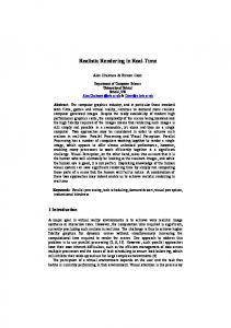
Fig. 1. High-level evaluation framework.

evidence that this second scenario may lead to better performance. We discuss how to extend our approach to include bus–bus communications in Section VI. Fig. 1 shows the high-level framework used in this paper to study routing in the proposed network. Our starting point is a simple mobility model for buses (described in Section III-B) that is supported by the statistical analysis of a set of real traces of the public transportation system of Turin, Italy, which serves an extended metropolitan area through about 7000 stops and 1500 vehicles distributed among 250 lines, with more than 4600 km of bus routes. These traces include the complete schedule for the morning rush hour period (6–10 A . M .) and the corresponding Global Positioning System traces for the vehicles belonging to 26 lines. A statistical analysis of these traces yields important conclusions, which allow us to appropriately represent the transportation system in terms of a graph with independent random weights, which we call the stop-line graph (see Section IV). Under this representation, our original optimization problem in identifying routes that maximize delivery probability by a given deadline (or maximize on-time delivery probability) becomes equivalent to a specific stochastic shortest path problem of the stop-line graph. We are able to find an optimal algorithm called O N -T IME for the single-copy case (see Section IV-B) and then to extend it for the multicopy case through a greedy approach (see Section IV-D). In Section V, we compare the performance of these proposed algorithms with three other heuristics (which is introduced in Section IV-C) that also operate on the stop-line graph, i.e., an adaptation of the routing algorithm proposed in [4] for bus–bus communications (we refer to it as M IN -H EADWAY), and the two naive algorithms M IN -D ELAY, which determines the path with the least expected traversal time, and M AX -P ROB, which maximizes the delivery probability on an infinite time horizon. Since the number of real-life traces that we obtained is limited, the comparison (see Section V) is based on simulations carried on a large set of synthetic traces generated on the basis of our bus mobility model and the schedule of Turin bus system. Additional material is presented in the Appendices. The proofs of the performance bounds for multicopy algorithms are in Appendix A. Appendix B presents an overview of bus mobility models in transportation literature, whereas Appendix C describes the algorithm that we propose to generate the synthetic traces based on the actual schedule of the transportation system. This paper provides the following main contributions: 1) Formulation of the original routing problem as a specific stochastic

shortest path problem on a particular stochastic graph (see Section IV-A). This formulation is justified by a statistical analysis of real transportation system traces (see Section III-B). 2) Optimal (under our model) routing scheme for the singlecopy case. While this offline routing scheme has, in theory, exponential worst-case time complexity, in practice, it is able to find the optimal route in a reasonable time, allowing each node to store an optimal preselected routing plan (see Section IV-B). 3) Extensions to the multicopy case, based on greedy approaches applied to the single-copy scheme. We prove a tight bound of 1/k for the on-time delivery probability in comparison to an optimal (nongreedy) k-copy scheme (see Section IV-D). 4) We derive an algorithm for generating mobility traces of the buses based on their actual schedule (see Appendix C). 5) Simulation analysis showing that the optimal algorithm mainly performs as M IN -D ELAY, whereas it outperforms M IN -H EADWAY and M AX -P ROB for reasonable values of packet-loss probabilities. We provide some explanation for these results. In this sense, the conclusion is that a naive algorithm such as M IN -D ELAY may be a very good heuristic for routing over realistic bus transportation networks (see Section V). 6) We present simulation results showing that only ten copies are needed for a multicopy greedy approach to achieve a performance similar to that of flooding, which requires at least two orders of magnitude more transmissions and copies for each single piece of data (see Section V-A). 7) We investigate of the effect of optimizing the location of the throwboxes covering many stops (see Section V-C). 8) We compare between bus-to-bus and bus-to-stop communication paradigms (see Section V-B). II. R ELATED W ORK Employing a bus network as a mobile backbone for dense vehicular networks was first proposed in [5], using standard routing protocols for mobile ad-hoc networks (e.g., DSR or AODV). More recently, the use of buses in a disconnected scenario has been considered, e.g., in the seminal DieselNet project [1]. Since our paper considers routing in such a network, in what follows, we only mention work related to routing issues. Appendix B will be devoted to discuss previous work on bus mobility models. Most of the research has focused on bus–bus communications [4], [6]–[9] with the following routing approach: Each vehicle learns at run time about its meeting process. Then, the vehicles exchange their local view with other vehicles and use the information collected to decide how to route data. The goals of the proposed algorithms were either to reduce the expected delivery time or maximize the delivery probability. Unlike these studies, we mainly focus on bus-to-stop data transfers and derive a single-copy routing algorithm to maximize the delivery probability by a given deadline. We then extend the algorithm to address settings where several copies of the same data are permitted. On the other hand, we do not consider buffer or bandwidth constraints (e.g., as in [6] and [7]) as they are not a major concern in our settings: When the mobile devices are buses (as opposed, for example, to cellular phones), it is

ACER et al.: TIMELY DATA DELIVERY IN A REALISTIC BUS NETWORK

reasonable to assume that there is sufficient storage available; in addition, since buses communicate with stops (as opposed to other moving buses), the amount of data transferable during a meeting is larger. Nevertheless, characterizing the bandwidth of the contacts and incorporating these constraints into our framework for bandwidth-hungry applications are part of our ongoing research. The use of fixed relay nodes was also considered in [2] and [10]. In [10], an architecture where bus passengers may use the cellular network to require content that will be delivered to access points along the bus trajectory is proposed. These data can also be replicated on other buses, taking advantage of possible data transfers between vehicles. Their analysis considers only a simplistic single-street scenario and does not address routing issues. Banerjee et al. [2] reported that the performance of a vehicular network is improved by adding some infrastructure, such as base stations connected to the Internet, a mesh wireless backbone, or fixed relays (which are similar to our stops). The most important results are given as follows: 1) There are scenarios where a mesh or relay hybrid network is a better choice over base station networks. 2) Deploying some infrastructure has a much more significant effect on delivery delay than increasing the number of mobile nodes. These findings, which were verified both analytically and by experiments on the DieselNet testbed, support our proposed architecture, which relies on opportunistic connectivity between vehicle nodes and fixed relays. To provide low-cost Internet connectivity to fixed kiosks in rural areas of developing counties, KioskNet architecture has been proposed [11]. In this architecture, buses carry data between the kiosks and gateways that are connected to the Internet. Routing of such data between the kiosks and the gateways is achieved by simple flooding. On the other hand, gateways are delegated to a kiosk via a scheduling mechanism that considers the schedule of the buses, which serve the kiosks [12]. The routing algorithms proposed by [13]–[16] are intrinsically more suited for bus-to-bus data transfers. Liu and Wu [14] and Liu et al. [16] proposed algorithms that take advantage of cyclic mobility patterns, according to which nodes periodically meet, albeit with some probability. Even if a given bus may meet multiple times the same stop, this approach does not fit our scenario for three reasons. First, the bus–stop contact process is not necessarily periodic, because vehicles may be assigned to different lines during one operation day. Second, even if a vehicle operates always on the same line, its frequency significantly changes along the day. Third and more importantly, even when a period may be defined, its value ranges from 30 min to 2 h, depending mainly on the length of the bus trajectory and on inactivity times at terminus. It is then comparable with the deadlines we are targeting, making it impossible to take advantage of such long-term periodicity. Other forms of long-term regularities in the contact process of the different nodes [15] are too general for our settings since we have significantly more information on the meetings that can be exploited to improve the performance. Finally, Liu and Wu [13] proposed hierarchical routing for a deterministic network, whereas we consider non-deterministic mobility.

1253

Almost all these papers previously mentioned have considered only small bus networks (40 buses for DieselNet and 16 buses on a cyclic path for MobTorrent [10]). Only [8] considers an urban setting with a public transportation system comparable with ours (70 different bus lines), but differently from us, they do not use any real mobility trace and simulate bus movement, assuming that the bus speed is uniformly chosen at random from a given interval. From the theoretical point of view, our optimization goal can be reformulated (under some assumptions) as a particular stochastic shortest path problem that deals with a graph whose edge lengths (or, equivalently, traversal times over the edges) are random variables. Several optimality criteria were considered in the past for routing in stochastic graphs. The most common one is the least expected traversal time, which can be generalized to any linear (or affine) utility function [17], [18]. Other optimality criteria are deviance [19], monotonic quadratic utility functions [20], and prospect-theory-based functions [21]. Recent and comprehensive surveys of the different utility functions and corresponding solutions appear in [22] and [23]. Our paper deals with the reliability of the chosen path, i.e., finding a path that maximizes the probability of on-time arrival (given some deadline). This problem was first studied by Frank [24] and then was also investigated in [25], [27], and, more recently, [22] and [28]–[30]. Current stateof-the-art algorithms still have exponential worst-case time complexity, based on enumerating over some set of candidate paths [22]. Our problem essentially differs from Frank’s problem in three aspects: First, we consider a real transportation system, and therefore, we are not interested in the worst-case complexity of the algorithm on some general graphs. Second, our transportation model has two kinds of entities, i.e., stations and buses; we need to take into account waiting time at the stops and not only buses travel times, as explained in detail in Section IV. Third, all the previous work considered a singlecopy model, whereas our model also deals with multiple copies, where the objective is that at least one of the copies arrives at the destination before the deadline. Finally, we observe that we use the bus network for data transfer as it is used for passenger transfer. Thus, one could expect that the same problem has already been addressed in the transportation literature. However, this is not the case: First, the possibility to exploit multicopy is clearly absent in the transportation of people or merchandise. Second, the probability to miss a transfer opportunity is also not considered in transportation, whereas data transfer between two nodes may fail because of insufficient contact duration, channel noise, or collisions. Third, even for single-copy routing, bus network passenger routes usually aim to minimize the expected traversal time (possibly limiting the maximum number of bus changes) and not to maximize the delivery probability by a given deadline, as we are doing (cf. [31]–[33] and references therein). The fact that finally minimizing the expected traversal time may provide almost optimal performance in some scenarios (when message transmissions do not fail) is an a priori unexpected finding of this research.

1254


In conclusion, to the best of our knowledge, this is the first paper that proposes an optimal routing algorithm that takes advantage of bus schedule information, as well as stochastic characterization of bus mobility, which is supported by real data traces.

III. M ODEL D EFINITIONS AND A SSUMPTIONS In this section, we formally define the terms and the notation we use to describe a transportation system, following the terminology used in transportation literature. A transportation system T has a set of stops denoted by S and a set of vehicles (buses) denoted by V, which travel between the stops according to a predetermined path and a predetermined schedule. For each vehicle v ∈ V, the schedule allows us to determine its trajectory denoted traj(v), which is the ordered sequence of stops that the vehicle traverses: traj(v) = (s0 , s1 , . . . sn ). In addition, each vehicle v is associated with a trip denoted trip(v), which is a time-stamped trajectory, i.e.,

trip(v) = ((s0 , τ0 ), (s1 , τ1 ), . . . (sn , τn ))

such that a vehicle v should arrive at stop si along its trajectory at time τi = τ (v, si ). We distinguish between the scheduled time τi and the actual time ti = t(v, si ), which is a random variable, depending on road traffic fluctuations, passengers boarding and alighting, etc. The difference between the actual arrival time at stop si , t(v, si ), and its corresponding scheduled arrival time τ (v, si ) is the lateness of the vehicle at stop si , l(v, si ): l(v, si ) = t(v, si ) − τ (v, si ). Note that the lateness is negative when the vehicle arrives earlier that its scheduled arrival. The delay between stops si and sj , i.e., d(v, si , sj ), is the change in lateness: d(v, si , sj ) = l(v, sj ) − l(v, si ). The time difference between the arrivals of a vehicle at two different stops si and sj is called the actual travel time between the two stops, tt(v, si , sj ) = t(v, sj ) − t(v, si ). The scheduled travel time is simply the difference between the scheduled arrivals at the two stops. A key concept in bus networks is the notion of lines, which are basically different vehicles with the same trajectory (at different times). Let L denote the set of lines. For each vehicle v ∈ V, we denote its corresponding line by line(v) = {v ∈ V | traj(v) = traj(v )}. Note that lines introduce an important characteristic of a bus transportation system: if a passenger misses a specific vehicle v, he/she can still catch another vehicle v in line(v) and reach the same set of stops. The time between two consecutive arrivals of vehicles belonging to the same line at the same stop is called headway. In the sequel, we will refer to the transportation system T as the quintuple S, V, L, τ (), t(), where function τ () is a way to represent the schedule and t() denotes a characterization of the stochastic process of vehicle arrivals at the stops. In the next section, we are going to start characterizing this stochastic process.

A. Communication Model We assume that a bus is able to communicate with the throwbox at the stop only when it comes close to the stop, i.e., it is in the transmission range of the throwbox. In our model, we do not explicitly introduce a departure time from the stop, because, in our paper, we do not take into account bandwidth constraints, and therefore, it is less important to specify the duration of the transmission opportunity between a bus and a stop. In practice, we assume the following: Assumption 1: Transmission opportunities are instantaneous and occur at the arrival time of the bus at the stop position. A drawback of this approach is that two overlapping transmission opportunities are artificially ordered and some transmission possibilities are lost. For example, if v1 and v2 can transfer to s in [t1 , t3 ] and in [t2 , t4 ], with t1 < t2 < t3 < t4 , respectively, data can be transferred in the two directions (from v1 to v2 and from v2 to v1 ), but when the transmission opportunities are ordered, only one direction is still feasible. Furthermore, we assume that data transfer during a transmission opportunity can fail. This can be due to different causes: not only channel noise and collisions but also nodes failing to discover the opportunity, or contact duration being insufficient to transfer the data. We assume the following: Assumption 2: Message success probabilities of different contacts are independent. B. Measurements on Bus Mobility and Their Implication The problem of maximizing the delivery probability by a given deadline requires realistic statistical characterization of bus mobility patterns, which is also useful in generating a large set of synthetic traces and evaluating the performance of our routing algorithms. Transportation literature does not provide a universally valid model for bus movements in an urban environment since they are strongly affected by vehicular and passenger traffic conditions, road organization (availability of separate lanes for buses), traffic signal control management (priority may be given to the approaching buses over the other traffic), company policies (penalties to the bus drivers for delays), and so on; details of our transportation literature survey are in Appendix B. Two extreme cases can be considered: 1) Buses that are late at one stop can always recover their delay at the following stop (speeding up and reducing their travel times). 2) Buses move almost in the same way, and they do not try to recover their delay. The first case better describes lines with high headway, whereas the second is probably more adapt for lines with short headways, where buses try to respect a given frequency, rather than an exact schedule.1 In terms of the quantities, we have previously defined, in the first case, that latenesses at consecutive stops are almost independent, whereas, in the second case, they are highly correlated. We have performed statistical analysis of a one-day trace with actual bus arrivals at their stops provided to us by Turin’s 1 This distinction is expressly advertised by a Turin public transportation system, with label lines as frequency based and schedule based.


Fig. 2.

1255

Autocorrelation functions for lateness, delay, and travel time.

public transportation company, which mainly operates not only buses but also trams and subway trains. The network consists of around 250 lines and a fleet of almost 1500 vehicles. Some manual inspection is needed to be able to assign a specific trip to their schedule (to evaluate metric like the lateness); therefore, we worked on a subset of the trace, which consists of 26 lines in both directions, with a total of 408 trips and 11 097 arrivals at bus stops. Fig. 2 shows the empirical autocorrelation function for lateness, delay, and travel time. In particular, we have considered for each vehicle the sequence of latenesses at consecutive stops2 (l(s0 ), l(s1 ), . . . , l(sn ), . . .), the sequence of delays between consecutive stops (d(s0 , s1 ), d(s1 , s2 ), . . . , d(sn , sn+1 ), . . .), and the sequence of travel times between consecutive stops (t1 − t0 , t2 − t1 , . . . , tn+1 − tn , . . .). We have assumed that the sequences (relative to the same quantity) obtained for different vehicles are samples of the same random process, and we have used them to evaluate the empirical autocorrelation function. Fig. 2 demonstrates that the lateness values at consecutive stops are highly correlated. It is then clear that a simplistic bus mobility model, where the actual arrival time of vehicle v at stop s is equal to the scheduled arrival time plus some noise that is independent from one stop to another (t(v, s) = τ (v, s) + n(v, s)), is unrealistic. At the same time, we note that delays and travel times are significantly less correlated; this suggests the following model in terms of travel time: t(v, sk ) = τ0 + l(s0 ) +

k

tt(v, si , si+1 )

(1)

i=0

where we can assume that travel times are independent random variables (and then also delays are independent). If we assume that delays are independent and identically distributed and that the lateness at the first stop l(s0 ) is distributed as d(si , si+1 ), it is possible to analytically evaluate the expression of the autocorrelation function. This is represented in Fig. 2 by the curve “theoretical lateness 1.” We note that there is still a strong part of the correlation to be justified. A specific analysis of the lateness at the first stop shows that l(s0 ) 2 With a slight abuse of notation, we omit the dependence on vehicle v, when it is clear from the context.

Fig. 3. Travel time distribution (aggregated and for different scheduled travel times).

is not distributed as d(si , si+1 ), and moreover, its variance is almost six times larger. This shows that the variability of vehicle departure times is a significant component of the variability of arrival times at following stops. If we correct the expression of the autocorrelation function taking into account this empirical finding, we can obtain the new curve “theoretical lateness 2” that matches the empirical one very well. As a conclusion of this statistical analysis, we assume the following in the rest of this paper: Assumption 3: Bus travel times at consecutive stops are independent (but not necessarily identically distributed; in particular, their distribution will depend on the corresponding scheduled value). We continue our statistical analysis by determining realistic distributions for the lateness at the first stop l(s0 ) and the delay distribution to completely characterize the random variables of (1). This also allows us to use this recursive formula to generate realistic random traces (see Appendix C for details). For example, Fig. 3 shows the empirical distribution of the travel times (assumed to be homogeneous across different lines) when all the samples are aggregated and when they are separated according to the corresponding scheduled travel times. It is evident that different distributions have to be used, depending on the different scheduled travel times. Since it is quite common in transportation literature to use lognormal distribution to model travel times (see Appendix B), we have accepted this assumption and characterized the parameters of the lognormal distributions for different scheduled travel times by momentmatching techniques. Our final assumption concerns the waiting time at a stop when commuting from one line to another: Assumption 4: The distribution of the waiting time at a stop only depends on the stop and the characteristic of the departing bus line and not on the arrival line. We note that Assumption 4, which plays an important role in enabling a graph representation with additive edge weights, is partially a consequence of Assumption 3. Indeed, consider

1256


buses moving according to the schedule and a passenger transferring from line 1 to line 2 at stop s. It is clear that the waiting time at the stop can be evaluated a priori on the basis of the scheduled arrival time of the 1 vehicle and the departure time of the following 2 vehicle. However, under Assumption 3, the arrival times of 1 buses at stop s are random variables, and so are the corresponding waiting times. Intuitively, if the variability of 1 arrival times is large3 in comparison to the headway of line 2 , the waiting time will have almost the same distribution of the waiting time seen by a Poisson observer; thus, it is independent of the 1 schedule.

Fig. 4. (a) Example of line-based graph Glines describing a bus network with stops S = {A, B, C, D, E, F } and lines L = {1, 2, 3, 4}. The node corresponds to a stop and the label on the edge represents the line connecting the two stops. (b) Corresponding line-stop graph Gsl . Dotted edges are travel edges, whereas dashed edges are travel-switch edges.

IV. ROUTING A LGORITHMS IN A B US N ETWORK As mentioned before, our routing algorithms aim to determine offline routes for the transportation system that maximize data delivery probability by a given deadline: Definition 1: Given a transportation system T = S, V, L, τ (), t(), a source stop ss , a destination stop sd , a start time tstart , and a deadline tstop , the on-time delivery problem is to find a route between ss and sd that starts after time tstart and maximizes the on-time delivery probability, i.e., Pr{data is delivered before time tstop }. We first discuss how we represent the transportation system as a graph, considering the natural operation of a bus system with transfers from buses to stops and then to buses (i.e., involving only bus–stop communications). The following four issues lead to our final graph representation: computational complexity, intrinsic properties of the bus transportation system (namely, the existence of lines), characteristic of the stochastic process t() (namely, waiting times at stops depend on the departing line), and an advantage coming from working with additive edge weights. For the sake of simplicity, in the following discussion, we will first consider that all the transmissions are successful. A. Graph Representation A simple way to represent the transportation system T is by a temporal network [34], which is a multigraph whose set of nodes consists of S ∪ V (i.e., a node for each vehicle and for each stop), and each edge represents a transmission opportunity between a vehicle v and a stop s (or vice versa) occurring at the time instant t(v, s) and can therefore be represented by the triple v, s, t(v, s) (or s, v, t(v, s)). A possible route in such graph would then be a path connecting the source ss and the destination sd , i.e., a sequence of edges, such as (ss , v0 , t(v0 , ss ), v0 , s1 , t(v0 , s1 ), s1 , v1 , t(v1 , s1 ), . . . , vn , sd , t(vn , sd )). This route is able to deliver the data from ss to sd , only if tstart ≤ t(v0 , ss ) ≤ t(v0 , s1 ) ≤ t(v1 , s1 ) ≤ · · · ≤ t(vn , sd ) ≤ tstop . While the temporal network is useful in general for deterministic scenarios, it is not suitable for the transportation system that we are considering. The first reason is that, in a largescale transportation network, this graph would have a very 3 Note that, according to our model, the variance of the lateness increases along the trajectory, and this condition tends to hold.

large number of nodes (|S ∪ V|) and of edges. For example, if the time interval [tstart , tstop ] spans a few hours, a stop in a dense traffic can exhibit hundreds of edges. The second reason is that it ignores the fact that, in a bus network, a vehicle in such route can be in some sense “replaced” by another vehicle of the same line. Finally, given our performance metric, we would need to evaluate Pr{tstart ≤ t(v0 , ss )) ≤ t(v0 , s1 )) ≤ t(v1 , s1 ) ≤ · · · ≤ t(vn , sd ) ≤ tstop }. However, the results of Section III-B show that lateness values at consecutive stops are strongly correlated, making it impossible to evaluate this probability in a simple way. For these reasons, it appears more beneficial to directly look for routes from the source to the destination in terms of lines. We can consider an alternative data structure, i.e., the line-based graph Glines = S, Elines , as shown in Fig. 4(a), in which nodes are bus stops and there is an edge between two stops si and sj if and only if there is a line ∈ L that goes from si to sj . (Only stops that are served by at least two lines need to be considered for relay purposes.) It is important to notice an intrinsic difference between the temporal network and the linebased graph: In the temporal network, we check the feasibility of the path by evaluating the probability that it maintains the chronological order between contacts. On the other hand, in the line-based graph, we are interested to check whether their total length (i.e., the total traversal time of the path) is less than tstop − tstart . Note that the traversal time along a specific path is a random variable, which is the sum of two kinds of random variables: 1) edge random variables, which capture how travel time between two specific stops on a specific line is distributed, and 2) node random variables, which capture the distribution of the waiting time at the stops. The waiting time at a stop poses a major difficulty on the design of a routing algorithm, because it is not simply related to the stop but it depends on the specific route under consideration and, more specifically, the stop’s outgoing and incoming edges in that route. For example, if both edges correspond to the same line, the waiting time at the stop is 0. On the other hand, when switching lines at the stop, the waiting time depends only on the headway of the departing line by Assumption 4. Hence, this graph is also not well suited for our purposes. In our proposed representation, which we call stop-line graph Gsl = Vsl , Esl , the nodes are (s, ) pairs, where s is a stop and is a line; (s, ) ∈ Vsl if and only if line ∈ L arrives at (or depart from) stop s ∈ S. In addition, we add two nodes


ss and sd , which are connected to all nodes that correspond to the source and destination stops. The edges of Gsl are defined as follows: An edge between (s, ) and (s , ) corresponds to traveling from stop s to stop s with line and then continuing from stop s on line . If = we call the edge a travel edge, whereas if = , we call it a travel-switch edge. An example of Gsl appears in Fig. 4(b). We now define the random variables associated to the edges in Esl . The random variable of a travel edge describes the corresponding travel time between two stops: formally, a travel edge e = ((s, ), (s , )) is associated with the random variable we = tt(, s, s ) describing the travel time of a line bus from stop s to stop s . The random variable of a travel-switch edge includes the travel time between the corresponding stops and the waiting time for the next line, taking into account possible transmission failures. Formally, a travel-switch edge e = ((s, ), (s , )) is associated with the following random variable we : we =

+∞, tt(, s, s ) + wt( , s , k),

with prob. pf with prob. (1 − pf )2 pk−1 f

1257

Fig. 5. Delivery probability cdfs of three disjoint paths P1 , P2 , and P3 connecting a source and a destination with different traversal times and without transmission failures (pf = 0). Path P1 has the lowest expected traversal time; the variance of P2 is the smallest, whereas P3 ’s variance is the largest. P1 , P2 , and P3 are the optimal paths computed by O N -T IME for deadlines between 34 and 43 min, larger than 43 min, and shorter than 34 min, respectively. The curve labeled P1 + P2 + P3 corresponds to the success probability obtained by a multicopy approach exploiting all the three paths concurrently.

B. Single-Copy Routing Algorithm and Implementation for any k ≥ 1; here, pf is the transmission failure probability, and wt( , s , k) is the waiting time at stop s before the arrival of the next kth bus of line . To explain the formula for we , note that, to be able to successfully forward the data from one bus to another, two transmissions must succeed, i.e., the one from a bus of to s (which may fail) and the one from s to a bus of (which will be successful after a geometric number of failures). The formula assumes that the transmission failure probability is the same for every possible transmission, but the model can be easily extended to consider the case where it depends on the stop and on the line to which the vehicle belong. We assume that all the random variables defining we are known (they will be characterized in Section IV-B); moreover, by Assumptions 3, 4, and 2, they are all independent. It is important to notice that the stop-line graph Gsl provides a unified approach to deal with waiting times at the stops, thus solving shortcoming in previous approaches (e.g., temporal network [34], or graphs with stops as nodes and lines as edges); furthermore, although out of the scope of this paper, Gsl is also usable in settings where Assumption 2 does not hold. Our model allows us to simply calculate the overalltraversal time of the data along a weighted path P as tr(P) = e∈P we . When transmission failures can occur, the cumulative distribution function (CDF) of the delivery time is scaled by a factor equal to (1 − pf ) for each transmission from a bus to a stop. Then, the cdf of the delivery time along a given route has the horizontal asymptote y = (1 − pf )m , where m is the total number of bus-to-stop transmissions in the route. Now, given graph Gsl , the on-time delivery problem corresponds with finding a path P from ss to sd such that Pr{tr(P) ≤ tstop − tstart } is maximized. Note that, under this construction, our problem is similar to the problem defined by Frank [24], with the differences highlighted at the end of Section II.

We now propose our routing algorithm called O N -T IME, which aims at solving the on-time delivery problem. O N -T IME finds, in general, different paths for different values of the (relative) deadline tstop − tstart . For example, Fig. 5 compares the cdfs for the delivery times of three different paths for a given source–destination pair and no transmission failures (pf = 0). In this case, O N -T IME chooses one of the three paths, depending on the given deadline. Nevertheless, the larger the deadline, the larger the resulting on-time delivery probability will be. O N -T IME works by first determining a potentially good path between the source and the destination (for example, that with the minimum expected traversal time) and evaluating its ontime delivery probability. This can be done by performing a (numerical) convolution of the different random variable distributions along the path, yielding the end-to-end traversal time distribution. By this distribution, it is then easy to calculate (using the corresponding cdf) the delivery probability by the deadline. Then, the algorithm proceeds by exploring the graph through a breadth-first search, looking for paths with a higher on-time delivery probability. A pruning mechanism avoids the need to determine and evaluate all the paths. Being that the traversal time is obtained by adding nonnegative link weights, for any path P and any prefix P of P, Pr{tr(P) ≤ t} ≤ Pr{tr(P ) ≤ t}. Thus, we can perform hop-by-hop convolution and compute, for each resulting distribution, the probability that the weight (i.e., the traversal time) of this path prefix is less than tstop − tstart ; if the probability is smaller than that of the current best path, there is no need to consider the rest of the path. From a practical point of view, working with a real transportation network, this simple pruning mechanism significantly reduces the number of paths to be considered, even if, theoretically, we may have a factorial number of paths to explore.

1258


In our implementation, we have introduced some other simplifications that reduce the computation time but, at the same time, may lead to suboptimal paths. First, we have introduced a limit h on the exploration depth during the search. Given h as a constant, the algorithm is then guaranteed to run in polynomial time. We observe that, upon termination, we may be able to say if the algorithm has selected the optimal path or there may be a better path. In fact, when we stop, if there is still a path prefix that the pruning mechanism cannot discard, then there could be a longer path with higher on-time delivery probability. However, if this is not the case, then the current best candidate is actually the optimal path. In our experiments on the Turin transportation network, h = 8 was enough to find all the best paths. Although this value may change for other networks, we think that it will remain a relatively small constant. Note that a suitable h for each network can be found by conducting experiments similar to ours. A second simplification is that we restrict the set of eligible paths such that each line can be used only in consecutive edges. This prevents the algorithm to explore paths using line 1 , then line 2 , and then again line 1 . We expect that these paths have normally worse performance than those where a data message just remains on line 1 . Finally, we have avoided the computation burden of performing numerical convolution by assuming that the end-to-end traversal time, which is a sum of independent random variables, can be approximated by a normal distribution. In this case, it is sufficient to take into account the mean and the variance of each edge weight, conditioned on the fact that it is finite (µe = E[we | we < ∞] and σe2 = Var[we | we < ∞], respectively) and the probability that the edge weight is finite (denoted by path P is equal to the pe ). Then, the cdf of the traversal time of cdf of a normal distribution with mean e∈P µe and variance 2 σ , multiplied by a scaling factor e∈P e e∈P pe . In the case of travel edges, the average and variance of tt(l, s, s ) can be directly estimated from the traces. In the case of travel-switch edges, we also have to evaluate the average and variance of wt(, s, k) using the first three moments of the interarrival times of the line buses to stop s (which can also be estimated from the traces) and some basic Palm calculus [35]. For example, assuming perfect periodic bus arrivals with period δ and failure probability pf , it can be shown that E [wt(, s, k)] = δ (1/2 + pf /(1 − pf )) E wt(, s, k)2 = δ 2 1/3 + 2pf /(1 − pf )2 . Note that these values can be computed for the specific arrival process observed in bus traces. In what follows, we evaluate the performance of O N -T IME for different source–destination pairs under similar kind of deadlines. If we had fixed a given deadline for all the pairs, then this deadline could be unfeasible for some of them (in the sense that there is no way to deliver the message by this deadline, e.g., if the deadline is smaller than the time that a vehicle would take to move from the source to the destination), and trivially satisfiable for other pairs. (Many different paths would deliver with probability almost one.) For this reason, given a source ss , a destination sd , and a real value x ∈ [0, 100], let φ(x, ss , sd )

be the deadline tstop for which the on-time delivery probability of the path from ss to sd with minimum expected traversal time is x% (assuming that pf = 0). We denote by ON-TIME(x) the on-time routing algorithm where the deadline is set equal to φ(x, ss , sd ) for every source–destination pair (ss , sd ). Intuitively, the smaller x is, the “shorter” the considered deadlines are, where “short” is in relation to the expected traversal time from ss to sd and not in an absolute sense. C. Other Routing Approaches Although the algorithm that we described is optimal under our model assumptions, we also consider suboptimal but simpler heuristics. The most intuitive approach (denoted as M IN -D ELAY) is to route in Gsl along the path whose expected traversal time is minimal. Note that, when the transmission failure probability is null, M IN -D ELAY is equivalent to O N -T IME(50) under the Gaussian assumption on the distribution of the traversal time. This is not true for different deadlines. For example, Fig. 5 shows that path P1 , which is found by M IN -D ELAY, does not always provide the highest on-time delivery probability. On the other hand, M IN -D ELAY is computationally attractive, because the path with the least expected traversal time can be easily computed with Dijkstra’s algorithm (by linearity of expectation). In Section V, we compare our optimal algorithm to this suboptimal heuristic and show that it often suffices to use this simple approach. A second algorithm, M AX -P ROB, selects the path that maximizes the delivery probability on an infinite time horizon. In addition, this path can be determined running Dijkstra’s algorithm on the line-stop graph with edge weights equal to − log(pe ). For high transmission failure probabilities, we can expect M AX -P ROB and O N -T IME to select the same path. At the end of Section V, we will show that this is the case. Another approach denoted as M IN -H EADWAY tries to minimize the sum of all lines headways along a path [4], thus preferring frequent lines over infrequent lines; it was originally proposed for bus-to-bus communications. In Section V, we show that it has the worst performance in our settings among all the different algorithms. D. Extension to Multicopy Routing As shown in the toy case of Fig. 5, using a multicopy scheme (the curve labeled “P1 + P2 + P3 ”) to simultaneously exploit several paths increases the on-time delivery probability to deliver the data within the deadline. In this specific example, path P2 becomes “useful” only for large deadlines, whereas P3 is “useful” for any deadline. We consider only multicopy schemes, such that at most k distinct copies of each data packet are present in the network at a given time instant. Without such a constraint, a flooding scheme that copies the data whenever there is a contact, i.e., in an epidemic manner, would achieve the best possible delivery probability. We propose a greedy Multicopy algorithm for on-time delivery problem that is denoted simply as MC-O N T IME. It


selects the k paths with the highest on-time delivery probability, without considering the interaction among them. This can be easily implemented by saving the best k paths while enumerating all possible paths as in O N -T IME. Moreover, our pruning mechanism is changed accordingly to compare the current path prefix with the kth best path discovered so far (rather than the best path). We can similarly extend the heuristics M IN -D ELAY, M AX -P ROB , and M IN -H EADWAY presented in Section IV-C to select the k paths with minimal expected traversal time, maximal success probability, and minimal total headway, respectively. Since our algorithm works in a greedy manner, it does not consider the interaction between the paths and, more specifically, the gain in probability over previously selected paths (which can be very small in case the paths overlap). This leads to theoretical performance degradation with respect to an optimal infeasible algorithm that considers the joint probability over all sets of paths. The following theorem, whose proof is in Appendix A, provides tight bounds on this performance degradation: Theorem 1: The MC-O N T IME algorithm always achieves at least 1/k of the on-time delivery probability of an optimal k-copy algorithm. In addition, there is a valid transportation graph for which MC-OnTime achieves at most (1/(1 − ε)k) of the on-time delivery probability of an optimal k-copy algorithm, for arbitrarily small ε > 0. The performance degradation is mainly due to path overlapping; consider two paths with high success probability that differ only in one edge: MC-O N T IME will choose both paths, whereas, in fact, the marginal gain in choosing the second path is small. Thus, we have also considered an algorithm that ensures that the paths are disjoint. That is, the MC-O N T IME -D ISJOINT algorithm iteratively chooses the path with the highest on-time delivery probability, among all paths from source to destination whose corresponding lines are not used by any previously selected path. However, we can show that the worst-case performance of MC-O N T IME -D ISJOINT is the same as that of MC-O N T IME. Moreover, some preliminary simulations have shown that MC-O N T IME is superior in practice, and therefore, this is the multicopy routing algorithm that we consider in the sequel.4 V. P ERFORMANCE E VALUATION We consider a set of 180 source–destination (ss −sd ) stop pairs among the 2550 stops inside the metropolitan area of Turin. In the first 90 pairs, both the source and the destination have been uniformly chosen at random in the entire metropolitan area; in the second 90 pairs, the source ss is located at a main transportation hub within the city center (close to the main train station of Turin), and all the destinations sd have been chosen uniformly at random. 4 MC-O N T IME -D ISJOINT and MC-O N T IME are two extremes as for the amount of overlapping between the paths. In our future research, we plan to also look on hybrid heuristics with strict bounds on the number of overlapping edges. While these variants yield the same (1/k) worst-case approximation, they might be proved superior in real-life traces.

1259

Fig. 6. Complementary cdf of the critical time window W guaranteeing on-time delivery probability ∈ [0.1,0.9] for the minimum expected traversaltime path.

To reduce deployment costs, we assume to employ one single throwbox covering close-by stops. Hence, stops are aggregated after setting the transmission range of each throwbox equal to 100 m; Section V-C discusses the effect of the transmission range on the total number of throwboxes to deploy. We generate a set of 100 traces with the parameters obtained by the statistical analysis. The traces include the trips of all vehicles of 250 bus lines for the four hours available from the schedule. Appendix C discusses in detail the trace generation process. We have developed a simulator that computes the delivery probability of each path by averaging across these 100 traces; note that the real-life trace alone would not be enough to compute this probability with any accuracy. Moreover, this trace includes only a small fraction of the lines in Turin, and the number of possible paths between a source and a destination using only this subset of lines is drastically reduced. Data are assumed to be available at the source stop at 7 A . M . As we mentioned in Section IV-B, for very short deadlines, there is probably no route that could deliver the packet with a reasonable probability, whereas, for very long deadlines, many different routes are able to deliver it with probability almost one (if all the transmissions succeed). Then, there exists an interval of deadline values for which it makes sense to “spend effort” to determine good routes. To quantify this interval, we introduce the “critical” time window of a route defined as W = φ(90) − φ(10): This is the amplitude of the interval of deadlines for which the route determined by O N -T IME(50) achieves delivery probabilities in [0.1,0.9]. Fig. 6 shows the {complementary} CDF of W , for the whole set of 180 pairs. For more than 90% of ss −sd pairs, the windows is larger than 10 min, and for more than 17% of them, it is even larger than 20 min. The maximum critical window size that we observed is 67 min. Then, for all 180 pairs and for all 100 traces, we evaluate the optimal paths found by the O N -T IME algorithm and compare their theoretical on-time delivery probability with the empirical one determined by simulations. We found a reasonable agreement, considering that there are some differences between the model and the synthetic traces. In fact, in our model, we considered a constant line frequency in the time period (whereas there

1260


Fig. 7. Delivery probability (average and 90% confidence interval) for two deadlines and different routing algorithms for reliable transmission (pf = 0). M IN -D ELAY is the same as O N -T IME(50).

are some small changes in the schedule and then in the synthetic traces) and the same headway distribution at each stop along the trajectory (whereas, for example, the headway variability is larger for the last stops than for the first stops). Moreover, in the synthetic traces, we made sure that two buses of the same line cannot overtake each other (see Appendix C for details). This introduces some further inhomogeneity that is not taken into account in the model. We start to compare the performance of the algorithms defined in Section IV, i.e., M IN -D ELAY, O N -T IME, M AX -P ROB, and M IN -H EADWAY, with the E PIDEMIC algorithm that floods the network by taking advantage of all the possible contacts (and, therefore, making very large number of copies). We first assume that transmissions are reliable, i.e., pf = 0. Recall that, in this case, M IN -D ELAY is equivalent to O N -T IME(50). We evaluate the actual on-time delivery probability of the best path obtained by each algorithm; for each pair ss −sd , we set the deadline to φ(x) for different values of x, and we compute the 90% confidence interval of the delivery probability, considering all the possible 180 pairs. We will report the results only for x = 10 (“short deadline”) and x = 50 (“average deadline”) since these cases are representative. Fig. 7 compares the delivery probability of the different algorithms for the two deadlines. The gain of E PIDEMIC with respect to all the other single-copy algorithms decreases as the deadline increases: E PIDEMIC achieves a delivery probability that is 3 times larger than O N -T IME for deadline φ(10) but only 1.5 times larger for deadline φ(50). Indeed, when the deadline is large enough, just one copy of the data is enough to reach 100% delivery probability. In such a case, E PIDEMIC does not introduce any gain in terms of performance, and the cost in terms of copies and transmissions is much larger than under single-copy algorithms. For example, we observed, on average, more than 600 copies for φ(10) and more than 900 copies for φ(50) under E PIDEMIC up to the deadline, whereas, for all single-copy algorithms, the number of transmissions for each data is, on average, 5.0 and always less than 12. O N -T IME(10) and O N -T IME(50) obtain the maximum delivery probability for deadline φ(10) and φ(50), respectively, as expected. However, comparing the corresponding confidence

Fig. 8. Delivery probability (average and 90% confidence interval) for O N T IME(50), M IN -D ELAY, and M AX -P ROB for deadline φ(50) and for different values of transmission failure probability pf .

intervals, they behave almost the same. A somewhat surprising result is that, in many cases (121 out of 180), O N -T IME(10) performs exactly as O N -T IME(50) (or, equivalently, as M IN -D ELAY). In fact, we verified by direct inspection that O N -T IME(10) and O N -T IME(50) select exactly the same optimal path. These results have also been confirmed for other deadline values: The optimal route is not very sensitive to the deadline. In most of the cases, the best path computed by O N -T IME(50) is the best for every deadline φ(x), with x ∈ [0,100]. Recall the example in Fig. 5, showing that the best path does, in general, depend on the deadline. Our experiments lead us to conclude that these cases are very rare in a real transportation system when transmissions always succeed. Thus, one can choose the path solely on the basis of the minimum expected travel time (i.e., the simple M IN -D ELAY algorithm), making it redundant to run the complex optimal algorithm O N -T IME. We now investigate the effect of transmission failures. Fig. 8 shows the delivery probability for different values of transmission failure probability pf . Even with failures, O N -T IME(50) and M IN -D ELAY similarly behave. Only when pf increases, M AX -P ROB shows an average delivery probability comparable to the two other algorithms; indeed, M AX -P ROB becomes more efficient when the transmission failures are high since the optimal policy tends to minimize the number of transmissions. Hence, all the algorithms appear to efficiently behave for large pf . A. Multicopy Routing We turn now to deal with multicopy settings. Fig. 9 shows the performance of the MC-O N T IME(x) policy, which takes advantage of the k paths with the highest delivery probability by the deadline φ(x). The figure shows the results obtained for all the 180 source–destination pairs, assuming reliable transmissions (pf = 0). For deadline φ(50), O N -T IME with one copy reaches a delivery probability that is about 66% of that achieved by E PIDEMIC, and a few more copies significantly reduces the performance gap. However, after ten copies, we observe only a negligible improvement. This is partially due


Fig. 9. Delivery probability (average and 90% confidence interval) versus the number of paths for deadline φ(50) and for multicopy routing and no transmission failures (pf = 0).

1261

portunities, only bus–bus communication opportunities, or both (referred to as all-all). In all cases, we consider that the message is generated by a user located at a main bus stop in Turin and copied to all the buses that go through the stop. To compare the message spreading speed in the different scenarios, we have considered the stops themselves as potential destinations. Fig. 10 shows the number of stops that are reached by a copy of the message over time. It appears that using bus–stop communications is more effective than using only buses and achieves almost the same performance of the all-all scenario. In particular, we observe that not all the stops can be reached when we rely only on buses without using the stops as fixed relays. On the contrary, the bus–bus communication scenario seems to be slightly faster immediately after the generation of the message. It is important to note that this evaluation neglects factors such as contact duration and physical/link layer constraints. Burgess et al. reported that the contact duration between two mobile nodes in a vehicular network may eventually be too short to transfer a message [6]. These effects are expected to be more significant in the bus–bus scenario when both nodes are mobile. On the contrary, in the bus–stop scenario, contact opportunities can be quite long because buses need to stop to let passengers board and alight. Hence, we expect that the performance gain of the bus–stop scenario in comparison to the bus–bus scenario increases when these other effects are considered. C. Bus Stop Aggregation

Fig. 10. Comparison of epidemic routing with bus–bus and bus–stop communications.

to the fact that MC-O N T IME exploits a given sequence of paths provided by the algorithms, whose internal “diversity” is limited. Furthermore, E PIDEMIC exploits low-probability paths that are efficient just for the specific trace instance considered in each simulation run; since the number of these low-probability paths can be very large, due to the redundant connectivity of the bus transportation system metropolitan area, there is a high probability that at least one of them will be used to deliver to the destination. Note that the cost in terms of transmissions and copies for E PIDEMIC (on average, more than 900) is at least one order of magnitude larger than the multicopy approach using a preselected subset of ten paths. B. Comparison of Bus-to-Bus Versus Bus-to-Stop Communications Prior work on bus-based delay-tolerant networks mainly has focused on exploiting opportunistic contacts between the buses. In our scenario, we utilize bus–stop contacts rather that bus–bus contacts. In this section, we provide a first comparison of the two approaches in terms of the speed of message propagation when flooding is used. Fig. 10 shows how fast epidemic routing diffuses a message in the network if it utilizes only stop–bus communication op-

An urban area transportation network typically contains a large number of stops. For example, there are 6868 stops in Turin, among which 2550 are in the metropolitan area. It may be unfeasible to install a throwbox at each of these stops. At the same time, this may not be necessary. In fact, many of these stops are close to each other, so that a single throwbox can be used to cover multiple of them. In this section, we quantify how many stops can be “aggregated,” in the sense that they are close enough to use a unique wireless box for all of them. One parameter used in aggregation is the communication range of wireless boxes dtx , and it is assumed to be homogeneous across all the stops. Two nodes are considered neighbors if their distance is less than dtx . We use a simple greedy heuristic algorithm to group close-by stops. Let N be the set of stops. We first pick the node, i.e., it sM , that has the largest number of neighbors. We place one wireless box at sM . Then, we remove sM and the neighbors of sM from N . We iterate this step until N is empty. The number of stop groups or the number of wireless boxes that should be installed to cover all the 6868 stops present in Turin is shown in Table I for different values of the transmission range; the reduction is evaluated as the ratio between the number of stops that does not need a throwbox and the total number of stops. As the communication range increases, a larger number of stops are grouped together. Hence, the number of wireless boxes required to provide coverage decreases, and the reduction ratio of the aggregation increases. We see that even a 100-m communication range can result in a large reduction

1262


TABLE I EFFECT OF AGGREGATING STOPS IN THE ENTIRE TOWN

TABLE II EFFECT OF AGGREGATING STOPS IN THE MAIN METROPOLITAN AREA

(almost 50%) in the number of throwboxes (i.e., in hardware cost) to deploy the bus-based DTN. Table II shows the effect of aggregation when only the 2550 stops in the metropolitan area of Turin are considered. Because the stops are more closely placed in the metropolitan area, the aggregation mechanism with the same transmission range results in a larger reduction ratio for the number of wireless access points that need to be deployed. VI. C ONCLUSION This paper has laid the foundations for a framework to analyze bus-based networks, where communication is between the mobile buses and the stops along their trajectories. Through a statistical analysis of traces taken from a real transportation system of a large urban area, we were able to obtain a succinct stochastic graph representation of the system and to devise routing algorithms on this graph. In addition, we were able to develop a synthetic trace generator, which, in turn, allowed us to perform an extensive simulation study, verifying the performance of our proposed algorithms. An important outcome of this study is that, although different from the optimal but computationally intensive algorithm, the simple M IN -D ELAY algorithm achieves excellent results in terms of success probability for any reasonable deadline, when transmissions succeed all the time. In addition, we show that increasing the number of data copies beyond 10 does not provide any meaningful boost in performance. As final comment, we note that our model can be extended to bus–bus communications by introducing some virtual stops located in correspondence to possible physical contact points between two different lines. By appropriate choice of weights on the corresponding edges (e.g., no waiting time and high failure probability), one can capture the nature of this kind of communication as well. The main challenge, which is left for future research, is to locate the physical contact points and bound their number so that the running time of the algorithm remains feasible. In future work, we also plan to extend our approach by releasing some or most of our assumptions discussed in Section III.

A PPENDIX A T IGHT B OUNDS ON THE P ERFORMANCE OF M ULTICOPY A LGORITHMS In this section, we provide the proof for Theorem 1 of Section IV-D, which deals with the performance of the multicopy MC-O N T IME algorithm. This algorithm computes the success probability of all paths in isolation and chose the k best paths (without considering the interaction between them). Theorem 1 comprises the following lower and upper bounds: Lemma 1: The MC-O N T IME heuristic always achieves at least 1/k of the success probability of an optimal k multicopy heuristic. Proof: Let p1 , . . . , pk be the success probability of the paths selected by the MC-O N T IME algorithm, such that pi corresponds to the path selected at iteration i. Let q1 , . . . , qk be the success probability of the paths selected by the optimal algorithm, and let Q1 , . . . , Qk be the corresponding events of successful delivery (i.e., Pr[Qi ] = qi ). Note that, by definition, p1 ≥ maxi qi . Thus k k

1 1 Pr[GREEDY succeeds] ≥ p1 ≥ qi ≥ Pr Qi k i=1 k i=1 =

1 Pr[The optimal algorithm succeeds] k

where the third inequality is due to the union bound. Lemma 2: There is a valid transportation graph for which MC-O N T IME achieves at most (1/(1 − ε)k) of the success probability of an optimal k multicopy algorithm, for arbitrarily small ε > 0. Proof: Consider a transportation graph in which, from the source to the destination, there are 2k paths. 1) k two-edge paths, which share their first edge. The probability to traverse this first edge is p, whereas the probability to traverse the second edge is 1 − ε/4. 2) k single-edge paths, such that the probability to traverse the edge is p(1 − ε/2). Assume that p = ε/((k−1)(1−(ε/2))2 ). The MC-O N T IME algorithm will choose the first k paths since p(1 − ε/4) > p(1 − ε/2). Since all these paths need to traverse the first edge, the probability that MC-O N T IME succeeds is at most p. On the other hand, the optimal algorithm will do better than the algorithm that chooses the last k paths. The inclusion–exclusion principle (a.k.a Bonferroni inequality) yields that the success probability of the optimal algorithm is at least k 2 kp(1 − ε/2) − p (1 − ε/2)2 . 2 This implies that the ratio between the success probability is at most

kp 1 −

ε 2

−

p k 2

p2

1−

ε 2 2

=

1 . k(1 − ε)


A PPENDIX B B US M OBILITY M ODELS IN T RANSPORTATION This investigation of the transportation literature is mainly based on the overviews in [36] and [37]. Some works provide probability distribution for arrival time or lateness or delay, based on empirical studies (e.g., [38]–[42]) or model simplification (e.g., [43] and [44]). Most studies use a skewed distribution for the lateness since it is more likely to be behind schedule than ahead. Lognormal or gamma random variables are the most common assumptions (see the summary table in [36]). About the statistical dependency of these quantities, contrasting effects hold. In general, once a bus with low headway is late at a given stop, it is difficult to recover its lateness. In fact, for lines with low headways, passengers usually do not regulate their arrival on the basis of the schedule. Hence, passenger arrival can be assumed to be a Poisson process. When a bus is late, the longer waiting time at following stops causes an increase in the number of passengers who board (and later alight), resulting in longer dwell times and higher and higher delay enroute. Therefore, lateness and delay are positively correlated in such cases: high lateness at a stop results in increased delay over the subsequent segment [38]. This phenomenon does not always occur on buses with higher headway. In fact, passengers now tend to arrive just before the scheduled departure time of desired bus. Hence, late buses do not board significantly more passengers than on-time buses. Furthermore, since higher headway buses often have slack built into their schedule, there is opportunity to recover some of the lost time [45]. Penalties to drivers for being excessively late encourage them to catch up to the schedule. Thus, the delay in a segment is negatively correlated with the lateness at the start of the segment. Because of these two phenomena, the delay on a bus line segment can either be negatively or positively correlated with the lateness at the start of the segment, depending on a large part on the line headway. Moreover, we observe that the lateness of a bus also has consequences on following buses on the same line and direction. A late bus boards more passengers, and so, it leaves less of them for the following bus. This effect would lead to a negative correlation between the lateness of consecutive buses. At the same time, in many cases, transport agency policies or traffic conditions make overtaking impossible or quite rare. Hence, a bus that is significantly late would also cause the consecutive buses to be late. Regarding dwell time, this can be a significant part of the total service time (up to 16% of the total service time according to [37]). This time clearly depends on the number of passengers boarding and alighting (empirical formulas are proposed in [46] and [47]) as well as on the crowding, fare types [40], payment modalities, bus design (separate/common doors for boarding and alighting), mode (i.e., bus or metro lines), and service type5 [48]. In addition, the contribution of dwell time to lateness correlation is not immediate. For example, a large dwell time can be due to a large number of passengers boarding 5 Service type can be rapid, limited, local, or combined, depending on the vehicle speed and the distance between consecutive stops.

1263

or alighting. In the first case, the alighting at following stops will be, in general, large and will be small in the second case. A PPENDIX C G ENERATION OF T UNABLE S YNTHETIC T RACES The real traces from Gruppo Torinese Trasporti (GTT) transportation network provide data about 26 lines that operate in the city. The variety in the traces allows us to model properties such as headway, travel time, and lateness. However, real traces cannot be used in performance evaluation because they cover only a small fraction of the lines in Turin, and the number of possible paths between a source and a destination using only this subset of lines is drastically reduced. In this case, we expect different routing algorithms to select the same path, and it would not be possible to really evaluate the potential gain—but also the computational complexity—of our approach in comparison to simpler ones. Moreover, we are interested to evaluate the best performance achievable by a bus-based DTN, and therefore, we want to consider a massive deployment of WiFi-enabled buses and stops in the metropolitan area. For these reasons, we have decided to rely on synthetic traces describing the mobility of all the buses in the network. In this section, we explain how these synthetic traces have been generated on the basis of our statistical analysis of the real data, as discussed in Section III. For each vehicle, we generate the sequence of the arrival times at the different stops in its trajectory according to (1), i.e., t(v, sk ) = τ0 + l(v, s0 ) +

k−1

tt(v, si , si+1 )

i=0

where τ0 is the scheduled departure time of the vehicle from the first stop; and the lateness at the first stop l(v, s0 ) and the travel times tt(v, si , si+1 ) are assumed to be independent random variables (see Section III). For the lateness at the first stop, we have assumed a triangular distribution with support [−2, +2] min, which resembles the empirical distribution that we observed. Travel times are assumed to have a truncated lognormal distribution, as it is common in transportation literature. The truncated lognormal distribution is completely characterized by its mean (MTT ), its variance (VTT ), and its maximum value (th). We have assumed that these quantities depend only on the corresponding scheduled travel time (ST T ). By trying to match the moments of the empirical distribution and the lognormal distribution, we have identified the following empirical relations: MTT = 0.7(ST T + 0.5) M2 VTT = TT 4 th = 2MTT .

[min]

(2)

[min2 ]

(3) (4)

Occasionally, we have been forced to artificially increase th to be able to guarantee the headway constraint (see below). The arrival times at the stops could be independently calculated for each bus generating the random variables l(v, s0 ) and tt(v, si , si+1 ) [whose parameters can all be evaluated from the

1264


schedule using (2) and (3)] and summing them according to (1) or, equivalently, in the following iterative way: t(v, s0 ) = τ0 + l(v, s0 ) (5) t(v, si ) = t(v, si−1 ) + tt(v, si−1 , si ). This procedure can produce synthetic traces where a bus can overtake another bus serving the same line, e.g., when the second is particularly late. This happens with higher probability the smaller is the headway of the line in comparison to the scheduled travel times. Being that we do not observe this phenomenon in the real traces, we want to also avoid it in the synthetic traces by introducing the headway constraint: buses belonging to the same line arrive at each stop in the same order. To satisfy such constraint while matching the empirical values for the first two moments (MTT and VTT ) for the travel time, we have introduced a “virtual queue” for each different distribution considered, i.e., one for each possible scheduled travel time value in the transportation network and one for the lateness at the first stop. Initially, such queues are all empty. The arrival times of buses belonging to the same line are orderly generated according to their schedules. Let t(vj , sk ) be the arrival time of the jth bus of a particular line at the kth stop. We want to guarantee that t(vj , sk ) > t(vi , sk ), for each j > i and for each k. All the random variables are generated and used as previously described as long as t(vj , sk ) > t(vj−1 , sk ). If this is not the case, a larger value is needed, and the last random variable is generated again until the condition is satisfied. If the random values generated and not used would be simply discarded, the actual distribution would be stochastically larger than the intended theoretical distribution. For this reason, all the values generated but not used are put in the corresponding queue, and we try to recycle them later. In fact, once a queue is no more empty, when a value from the corresponding distribution is needed to generate a new arrival time, e.g., t(vl , sh ), it will be taken among those in the queue that are large enough to guarantee that the bus order is respected, i.e., that t(vl , sh ) > t(vl−1 , sh ). If the associated queue is empty, a new value is generated as previously described (and possibly added to the queue if it is not large enough). If the number of values in each queue at the end of the trace generation is small, the distortion between the actual and theoretical distributions is small. In our case, we have observed that, at the end of each trace generation, only a small number of values (less than 0.7%) remains in the queues in comparison with the total number of generated random variables. ACKNOWLEDGMENT The authors would like to thank both Dr. F. Arneodo and Dr. R. Aguilar from Tecnologie Telematiche Trasporti Traffico Torino (5T) for the traces that they provided and their availability to explain and discuss the details of the Turin public transportation system. R EFERENCES [1] UMass DieselNet Research. [Online]. Available: http://prisms.cs.umass. edu/dome/umassdieselnet [2] N. Banerjee, M. D. Corner, D. Towsley, and B. N. Levine, “Relays, base stations, and meshes: Enhancing mobile networks with infrastructure,” in Proc. ACM Mobicom, San Francisco, CA, Sep. 2008, pp. 81–91.

[3] V. Cerf, S. Burleigh, A. Hooke, L. Torgerson, R. Durst, K. Scott, K. Fall, and H. Weiss, RFC 4838: Delay-Tolerant Networking Architecture. [Online]. Available: http://tools.ietf.org/html/rfc4838 [4] M. Sede, X. Li, D. Li, M.-Y. Wu, M. Li, and W. Shu, “Routing in large-scale buses ad hoc networks,” in Proc. IEEE WCNC, 2008, pp. 2711–2716. [5] K. J. Wong, B. S. Lee, B. C. Seet, G. Liu, and L. Zhu, “Busnet: Model and usage of regular traffic patterns in mobile ad hoc networks for intervehicular communications,” in Proc. ICT Conf., 2003, pp. 273–289. [6] J. Burgess, B. Gallagher, D. Jensen, and B. N. Levine, “MaxProp: Routing for vehicle-based disruption-tolerant networks,” in Proc. IEEE INFOCOM, Apr. 2006, pp. 1–11. [7] A. Balasubramanian, B. Levine, and A. Venkataramani, “Dtn routing as a resource allocation problem,” SIGCOMM Comput. Commun. Rev., vol. 37, no. 4, pp. 373–384, Oct. 2007. [8] S. Gaito, D. Maggiorini, E. Pagani, and G. P. Rossi, “Distance vector routing for public transportation vehicular networks: Performance evaluation on a real topology,” in Proc. 2nd IFIP Wireless Days Conf., Paris, France, 2009, pp. 1–5. [9] F. Giudici, D. Maggiorini, and G. P. Rossi, “Performance evaluation of routing protocols for public transportation vehicular networks,” in Proc. 1st IFIP Wireless Days Conf., Dubai, United Arab Emirates, 2008, pp. 1–5. [10] C. B. Bin and C. M. Chan, “MobTorrent: A framework for mobile Internet access from vehicles,” in Proc. INFOCOM, 2009, pp. 1404–1412. [11] S. Guo, M. H. Falaki, U. Ismail, E. A. Oliver, S. U. Rahman, A. Seth, M. A. Zaharia, and S. Keshav, “Design and implementation of the Kiosknet system (extended version),” David R. Cheriton School Computer Science, Univ. Waterloo, Waterloo, ON, Canada, Tech. Rep. CS2007-40, 2007. [12] S. Guo and S. Keshav, “Fair and efficient scheduling in data ferrying networks,” in Proc. ACM CoNEXT, New York, 2007, pp. 1–12. [13] C. Liu and J. Wu, “Scalable routing in delay tolerant networks,” in Proc. 8th ACM Int. Symp. Mobile ad hoc Netw. Comput., Montreal, QC, Canada, 2007, pp. 51–60. [Online]. Avialable: http://portal. acm.org/citation.cfm?id=1288107.1288115 [14] C. Liu and J. Wu, “Routing in a cyclic mobispace,” in Proc. 9th ACM Int. Symp. Mobile ad hoc Netw. Comput., Hong Kong, 2008, pp. 351–360. [Online]. Available: http://portal.acm.org/citation.cfm?id=1374665 [15] C. Liu and J. Wu, “An optimal probabilistic forwarding protocolin delay tolerant networks,” in Proc. 10th ACM Int. Symp. Mobile ad hoc Netw. Comput. MobiHoc, New York, 2009, pp. 105–114. [16] C. Liu, J. Wu, and I. Cardei, “Message forwarding in cyclic mobispace: The multi-copy case,” in Proc. 6th IEEE Int. Conf. MASS, 2009, pp. 413–422. [17] S. T. Waller and A. K. Ziliaskopoulos, “On the online shortest path problem with limited arc cost dependencies,” Networks, vol. 40, no. 4, pp. 216–227, Dec. 2002. [18] J. S. Provan, “A polynomial-time algorithm to find shortest paths with recourse,” Networks, vol. 41, no. 2, pp. 115–125, Mar. 2003. [19] S. D. Boyles, “Reliable routing with recourse in stochastic, timedependent transportation networks,” M.S. thesis, Univ. Texas at Austin, Austin, TX, 2006. [20] S. D. Boyles and S. T. Waller, “The impact of nonlinear objective functions in online shortest paths,” in Proc. 86th Annu. Meeting Transp. Res. Board, 2007. [21] D. Kahneman and A. Tversky, “Prospect theory: An analysis of decision under risk,” Econometrica, vol. 47, no. 2, pp. 263–291, Mar. 1979. [22] Y. M. Nie and X. Wu, “Shortest path problem considering on-time arrival probability,” Transp. Res. B, Methodol., vol. 43, no. 6, pp. 597–613, Jul. 2009. [23] S. D. Boyles, “Operational, supply side uncertainty in transportation networks: Causes, effects, and mitigation strategies,” Ph.D. dissertation, Univ. Texas at Austin, Austin, TX, 2009. [24] H. Frank, “Shortest paths in probabilistic graphs,” Oper. Res., vol. 17, no. 4, pp. 583–599, Jul./Aug. 1969. [25] P. B. Mirchandani, “Shortest distance and reliability of probabilistic networks,” Comput. Oper. Res., vol. 3, no. 4, pp. 347–355, Dec. 1976. [26] E. Miller-Hooks, “Optimal routing in time-varying, stochastic networks: Algorithms and implementations,” Ph.D. dissertation, Univ. Texas at Austin, Austin, TX, 1997. [27] E. Miller-Hooks and H. Mahmassani, “Path comparisons for a priori and time-adaptive decisions in stochastic, time-varying networks,” Eur. J. Oper. Res., vol. 146, no. 1, pp. 67–82, Apr. 2003. [28] Y. Fan, R. Kalaba, and J. Moore, “Arriving on time,” J. Optim. Theory Appl., vol. 127, no. 17, pp. 497–513, Dec. 2005.


[29] Y. Fan and Y. Nie, “Optimal routing for maximizing the travel time reliability,” Netw. Spatial Econ., vol. 6, no. 3, pp. 333–344, Sep. 2006. [30] Y. A. Nie, “Arriving-on-time problem: Discrete algorithm that ensures convergence,” Transp. Res. Rec. J. Transp. Res. Board, vol. 1964, no. 1, pp. 193–200, 2006. [31] S. Vivas and G. Riano, “Mobile device programming for finding optimal path on a fast-bus system,” in Proc. IEEE SIEDS, 2006, pp. 196–201. [32] J. Boyan and M. Mitzenmacher, “Improved results for route planning in stochastic transportation networks,” in Proc. Symp. Discrete Algorithms, 2001, pp. 895–902. [33] M. Datar and A. G. Ranade, “Commuting with delay prone buses,” in Proc. Symp. Discrete Algorithms, 2000, pp. 22–29. [34] D. Kempe, J. Kleinberg, and A. Kumar, “Connectivity and inference problems for temporal networks,” J. Comput. Syst. Sci., vol. 64, no. 4, pp. 840–842, Jun. 2002, Special issue on STOC 2000. [35] F. Baccelli and P. Bremaud, Elements of Queueing Theory: Palm Martingale Calculus and Stochastic Recurrences.. New York: Springer-Verlag, 2010. [36] M. Dessouky, A. Singh, and R. Hall, “Transit ITS Simulator (TRANSITS): Design Document,” Univ. California, Berkekey, CA, Tech. Rep. UCB-ITS-PWP-97-26, 1997. [37] R. L. Bertini and A. M. El-Geneidy, “Modeling transit trip time using archived bus dispatch system data,” J. Transp. Eng., vol. 130, no. 1, pp. 56–67, 2004. [38] M. A. Turnquist, “A model for investigating the effect of service frequency and reliability on bus passenger waiting times,” Transp. Res. Rec., vol. 663, pp. 70–73, 1978. [39] W. Talley and A. Becker, “On-time performance and the exponential probability distribution,” Transp. Res. Rec., vol. 1108, pp. 22–26, 1987. [40] R. Guenthner and K. Hamat, “Distribution of bus transit on-time performance,” Transp. Res. Rec., vol. 1202, pp. 1–8, 1988. [41] P. N. Seneviratne, “Analysis of on-time performance of bus service using simulation,” J. Transp. Eng., vol. 116, no. 4, pp. 517–531, 1990. [42] J. G. Strathman and J. R. Hopper, “Empirical analysis of bus transit on-time performance,” J. Transp. Eng., vol. A27, no. 2, pp. 93–100, Apr. 1993. [43] P.-A. Andersson and G.-P. Scalia-Tomba, “A mathematical model of an urban bus route,” Transp. Res. B, Methodol., vol. 15, no. 4, pp. 249–266, Aug. 1981. [Online]. Available: http://ideas.repec.org/ a/eee/transb/v15y1981i4p249-266.html [44] R. W. Hall, “Vehicle scheduling at a transportation terminal with random delay en route,” Transp. Sci., vol. 19, no. 3, pp. 308–320, Aug. 1985. [45] R. Hall, M. Dessouky, A. Nowroozi, and A. Singh, “Evaluation of ITS technology for bus timed transfers,” Univ. Calif., Berkekey, CA, Tech. Rep. UCB-ITS-PRR-97-37, 1997. [46] H. Levinson, “Analyzing transit travel time performance,” Transp. Res. Rec., vol. 915, pp. 1–6, 1983. [47] R. Guenthner and K. Sinha, “Modeling bus delays due to passenger boardings and alightings,” Transp. Res. Rec., vol. 915, pp. 7–13, 1983. [48] T. Lin and N. H. Wilson, “Dwell time relationships for light rail systems,” Transp. Res. Rec., vol. 1361, pp. 287–295, 1992.

Utku Günay Acer (M’09) received the B.S. (honors) degree in telecommunications engineering from Sabanci University, Istanbul, Turkey, in 2004 and the M.S. and Ph.D. degrees from Rensselaer Polytechnic Institute, Troy, NY, in 2005 and 2009, respectively. From 2009 to 2010, he was a Postdoctoral Researcher with the National Research Institute of Informatics and Control, Sophia-Antipolis, France. He is currently a Researcher with Alcatel-Lucent Bell Laboratories, Antwerp, Belgium.

1265

Paolo Giaccone (M’98) received the Dr.Ing. and Ph.D. degrees in telecommunications engineering from Politecnico di Torino, Turin, Italy, in 1998 and 2001, respectively. During the summer of 1998, he was with the High Speed Networks Research Group, Lucent Technology–Bell Labs, Holmdel, NJ. During 2000–2001 and in 2002, he was with the Information Systems Networking Laboratory, Department of Electrical Engineering, Stanford University, Stanford, CA. He is currently an Assistant Professor with the Dipartimento di Elettronica, Politecnico di Torino. His research interests include the design of network algorithms, the theory of interconnection networks, and the performance evaluation of telecommunication networks through simulative and analytical methods.

David Hay (M’09) received the B.A. (summa cum laude) and Ph.D. degrees in computer science from Technion–Israel Institute of Technology, Haifa, Israel, in 2001 and 2007, respectively. Prior to joining Hebrew University, Jerusalem, Israel, he was with IBM Haifa Research Labs, Haifa (1999–2002); Cisco Systems (2006); Ben-Gurion University of the Negev, Beersheba, Israel (2007–2008); Politecnico di Torino, Turin, Italy (2008–2009); and Columbia University, New York, NY (2009–2010). He is currently a Senior Lecturer (Assistant Professor) with the Rachel and Selim Benin School of Computer Science and Engineering, Hebrew University. His research interests are algorithmic aspects of high-performance switches and routers in particular, quality-of-service provisioning, competitive analysis, and packet classification.

Giovanni Neglia (M’02) received the Master’s degree in electronic engineering and the Ph.D. degree in telecommunications from the University of Palermo, Palermo, Italy, in 2001 and 2005, respectively. In 2005, he was a Research Scholar with the University of Massachusetts, Amherst, visiting the Computer Networks Research Group. Before joining the National Research Institute of Informatics and Control (INRIA), Sophia-Antipolis, France, as a permanent member in September 2008, he became a Postdoctoral Researcher with the University of Palermo in June 2005 and an External Scientific Advisor with the Maestro team in September 2006. He is currently a Researcher with the Maestro team, INRIA. To this end, he applies different mathematical tools (Markov processes, control theory, fluid models, game theory, and gradient-based and metaheuristic optimization). His research interests include modeling and performance evaluation of computer networks and proposals of new mechanisms to improve their performance.

Saed Tarapiah received the B.Sc. degree in computer engineering from An-Najah National University, Nablus, Palestine, in 2005 and the M.Sc. and Ph.D. degrees in telecommunications engineering from Politecnico di Torino, Turin, Italy, in 2007 and 2011, respectively. In 2007, he was member of the AROMA project at Telecom Italia labs, TIM Turin. During 2009–2010, he was with MAESTRO Team, the National Research Institute of Informatics and Control (INRIA) (Mediterrane Research Centre). He is currently an Assistant Professor with the Department of Communication Engineering, AnNajah National University. His research interests include network coding in ad hoc networks, routing in delay-tolerant networks, and the encryption and security in ad hoc networks.