Tissue Perfusion diagnostic classification using a ... - Semantic Scholar

Tissue Perfusion diagnostic classification using a Spatio-Temporal Analysis of Contrast Ultrasound Image Sequences Quentin Williams1 , J. Alison Noble1 , Alexander Ehlgen MD2 , and Harald Becher MD2 1

Wolfson Medical Vision Lab, University of Oxford, UK, {quentin,noble}@robots.ox.ac.uk, WWW home page: http://www.robots.ox.ac.uk/~mvl/ 2 John Radcliffe Hospital, Oxford, UK,

Abstract. The analysis of tissue perfusion in myocardial contrast echocardiography (MCE) remains a qualitative process dependent on visual inspection by a clinician. Fully automatic techniques that can quantify tissue perfusion accurately has yet to be developed. In this paper, a novel spatio-temporal technique is described for segmenting the myocardium into differently perfused regions and obtaining quantitative perfusion indices, representing myocardial blood flow and blood flow reserve. Using these indices, Myocardial segments in 22 patients were classed as either healthy or diseased and results compared to coronary angiogram analysis and an experienced clinician. The results show that the automatic method works as well as a human at detecting areas of ischaemia, but in addition localizes the spatial extent of each perfused region as well. To our knowledge this is the first reported spatio-temporal method developed and evaluated for MCE assessment.

1

Introduction

The evaluation of tissue perfusion in various parenchymatous organs is important in the diagnosis, determination of severity, and localisation of ischemic disease. In echocardiography, the assessment of myocardial perfusion by means of ultrasound contrast agents is a valuable adjunct to wall motion analysis although considered today of secondary importance in terms of automatic quantification. The literature in this area is surprisingly sparse although clinically there is great interest in perfusion assessment, as perfusion abnormalities are an earlier indicator of coronary disease than abnormal wall motion. Both quantitative and qualitative measurements of tissue perfusion can be made by injecting a contrast agent (microbubbles) intravenously and then imaging the changes in signal intensity as the contrast agent makes its pass through an organ. This has permitted the application of myocardial contrast echocardiography (MCE) to the evaluation of myocardial blood flow and, thus, detection of obstructive coronary artery disease([1–3]). However, interpretation of MCE

studies have mostly been qualitative and subjectively based upon a clinician’s visual inspection of the image sequences. Recent advances in contrast ultrasound have made it possible to develop quantitative analysis systems capable of extracting clinical meaningful information from MCE studies. These are mostly based on the destruction-replenishment principle introduced by Wei et al. [4]. During a constant intravenous infusion of a contrast agent the microbubbles within the myocardium are depleted using high power ultrasound (mechanical index = 1.0) and their replenishment is assessed using low power ultrasound (mechanical index = 0.1). The replenishment kinetics allow the calculation of myocardial blood flow by estimating blood volume and mean blood velocity within the regions of interest (ROI) placed in the myocardium. Linka et al. ([5]) took the processing a step further by analysing replenishment curves within the entire left ventricular myocardium and displaying the calculated parameters (blood flow, blood volume and mean blood velocity) with different hues in parametric colour maps. Each parameter is displayed in a separate image whose colours display the quantities calculated by the replenishment model. Lower colour hues will indicate lower perfusion rates, and elucidate possible diseased areas. However, these semi-automatic techniques still require user intervention and visual interpretation, while they suffer from ad hoc smoothing in space and time. Recently, we have developed a new approach for perfusion quantification ([6]) in which a novel spatio-temporal method is used to classify the MCE sequences into different regions of perfusion. Classification is done by analysing the temporal pattern of relationships between pixels in a global manner, using a Bayesian Factor Analysis (BFA) model, and incorporating spatial information through a Markov Random Field (MRF). That paper presented only a preliminary version of the algorithm and no clinical validation. This paper, however, goes on to further develop the quantification algorithm and shows how the BFA-MRF method can be used to obtain quantitative perfusion indices that can aid the clinician in the diagnosis and assessment of diseased tissues. Two different indices, blood flow and blood flow reserve, are extracted for each region and used to identify the region as normal, abnormal or nondiagnostic. A clinical validation of the methodology based on 22 patient studies, is also presented, and the results are compared to coronary angiogram analysis as well as diagnosis from a clinician experienced in MCE. The results show that the automatic method works as well as a human at detecting areas of ischaemia, but in addition localizes the spatial extent of each perfused region as well.

2 2.1

Methods Image Data

All patients were referred to the John Radcliffe Hospital for standard dobutamine stress echocardiography for evaluation of inducible ischemia. Only patients, with a scheduled coronary angiogram were included in this study. 12 patients had a

normal angiogram or insignificant coronary artery disease and 10 patients showed various degrees of stenosis (>50%) in one or more of the three main coronary arteries. All datasets were obtained using the replenishment principle of Wei et al. [4] R (Bracco during a constant intravenous infusion of the contrast agent SonoVue International B-V). The contrast agent is routinely used in our hospital to enhance the endocardial border for wall motion analysis and to assess myocardial perfusion visually. Images were acquired using the real-time Power Modulation technique on the SONOS5500 ultrasound machine (Philips, Andover, MA, USA) and afterwards transferred to a computer for off-line analysis. Here, image sequences were cut according to the acquired ECG to keep just end-systolic (end of T-wave) frames and to extract the replenishment sequence. In this study, only standard apical views were used to evaluate the replenishment sequences (apical 4-chamber view, apical 2-chamber view, and apical long-axis view) to allow visualisation of the entire left ventricular myocardium and to minimise artefacts. Images were included into the study if the entire myocardium was visible, free of severe artefacts, and the cavity sufficiently opacified. Most MCE sequences were acquired at peak stress and therefore only 8 rest sequences were available. These resulted in 50 different image sequences consisting of various apical 4-chamber views (4 at rest and 21 at stress), apical 2-chamber views (1 at rest and 9 at stress) and apical long axis views (3 at rest and 11 at stress). For the automatic algorithm analysis, half the image sequences available in each view were randomly selected to form a control group of 25, with the remaining used as a test group. This was done so that the quantification measures could be trained on the control group and then ’blindly’ tested on the remaining 25. 2.2

Clinical reference

The reference (ground truth) for this study was coronary angiography with visually assessed stenosis >50% quoted as abnormal. The left ventricular myocardium for each dataset was divided using the 16-segment anatomical heart model proposed by the American Society of Echocardiography [13] (i.e. each wall was sub-divided in an apical, mid and basal segment). The same model was used to assign each segment to one of the 3 major coronary arteries (LAD, LCX, RCA) as is the clinical practice for assessing heart function. If coronary angiography revealed abnormality in the assigned artery, the segment was designated abnormal and normal otherwise. In total 246 myocardial segments were tagged in this manner. Although there is tremendous variability in the coronary artery blood supply to myocardial segments, it was felt appropriate to assign indivual segments to coronary artery territories to allow for standardisation and comparison to the other methods. An experienced MCE reader (AE) analysed each dataset qualitatively by visual assessment of myocardial perfusion during the replenishment sequence, and scored each segment as normal, abnormal or non-diagnostic. The MCE reader was completely blinded to any patient information and the outcome of the coro-

nary angiogram. The image quality of each dataset was also graded by the MCE reader as poor, medium or high. 2.3

Review of Automatic BFA-MRF method

We have previously proposed a novel spatio-temporal technique to assess tissue perfusion by automatically classifying the ultrasound images into different regions of perfusion. This Bayesian Factor Analysis - Markov Random Field (BFAMRF) method is described in detail in [6], and is summarized below. Briefly, it treats the classification as a statistical problem, which involves assigning to each pixel a class label taking a value from the set L = {1, 2, . . . , l}, where each pixel is indexed by a two-dimensional rectangular lattice S = {1, 2, . . . , n} and characterised by a p-variate vector of intensity values yi = {yi1 , . . . , yip }, i ∈ S. In this case each observation vector yi represents an intensity-time curve for a single pixel location. The problem of classification is then to estimate the true but unknown labeling configuration, x∗ , given the observed intensity time vectors, Y′ = {y1 , . . . , yn }. In particular, the maximum a posteriori (MAP) estimate of x is used: x ˆ = arg max{P (Y|x)P (x)}. (1) x∈X

The right-hand side of the above equation contains two parts: P (Y|x) and P (x), which are defined as a Bayesian Factor Analysis likelihood distribution and a Markov Random Field prior distribution, respectively. What remains is the estimation of the parameters of these two distribution functions, where the BFA model is constructed as a generative latent variable model, (yi |(µ, Λ, fi ) = µ + Λfi + ǫi ,

(2)

for each observation vector yi (i = 1, . . . , n), where µ is the overall population mean, Λ is a matrix of constants called the factor loading matrix; fi = (fi1 , . . . , fil ), is the factor score vector for pixel i; and the ǫi ’s are noise variables assumed to be mutually uncorrelated and Normally distributed N(0,Ψ). The factor loading matrix, Λ, expresses how each latent factor loads onto the observed variables, therefore giving an indication of how the hidden factors might look. In the case of a perfusion study, each column in the factor loading matrix will represent an intensity-time curve associated with each different type of perfusion present in the dataset. The factor scores give the estimated value (“weight”) of the observations on the hidden factors. Therefore, if each hidden factor represents a class, the factor score vector gives an indication of how much an observation belongs to each class. Since the parameters µ, Λ, the fi′ s, and Ψ are all unobservable, a Normal likelihood distribution for each yi is assumed, and written as: p

1

1

′

p(yi |µ, Λ, fi , Ψ) = (2π)− 2 |Ψ|− 2 e− 2 (yi −µ−Λfi ) Ψ

−1

(yi −µ−Λfi )

.

(3)

The probability of an MRF realisation, x, is given by the Gibbs distribution: P (x) = Z −1 e(−ωU (x)) ,

(4)

where U (x) =

X

Vc (x)

(5)

c∈C

is the energy function which is a sum of clique potentials Vc (x) over all possible cliques C. Z is a normalisation term and ω is a positive constant which controls the size of clustering. The potential function used is, Vc (xi ) = −δxi =x′i where δxi =x′i = 1, if xi = x′i , and 0 otherwise. The novelty of this particular algorithm stems from the way it interlinks the factor scores in the BFA model to the prior probability of the MRF model. The factor score vector indicates how much an observation belongs to a particular class. It is therefore assumed that the prior probability of the factor scores matrix, F′ = (f1 , . . . , fn ), follows the same prior probability of the classification configuration, x, and in fact that the factor score for each hidden factor (or class) is equivalent to the posterior probability of the class label. For every l ∈ L and i ∈ S fil = P (yi |l)P (xi = l). (6) Using the prior probability (4) and the likelihood function (3) with respect to xi and fil gives p

1

1

′

fil = Z −1 e(−ωU (xi )) × (2π)− 2 |Ψ|− 2 e− 2 (yi −µ−Λl fil ) Ψ

−1

(yi −µ−Λl fil )

.

(7)

Therefore the posterior probability values obtained through the MRF-MAP classification can directly be used as the factor scores. Thus, the strategy underlying this algorithm can be summarized as follows: (1) With the Gibbs function estiˆ , using the current estimate of the parameters; mate the labelling configuration, x (2) use it to specify the factor scores matrix, F; (3) and then estimate the new values of the parameters µ, Λ , and Ψ, using an iterative conditional modes (ICM) approach as described in [6]. These steps are iteratively repeated until suitable convergence is reached. The BFA-MRF algorithm was initiated using a simple K-Means Clustering method that provides the initial estimate for the ˆ . The algorithm was implemented in a multiscale framelabelling configuration, x work to improve convergence, first executed at a 1/4 of the resolution, then at 1/2, and finally at full resolution.

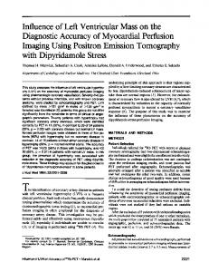
Fig. 1. Frames 1, 3 and 12 of a 4-chamber image sequence and the classification result. White = normal, Gray = abnormal, black = cavity.

Fig. 2. Frames 3, 7 and 8 of a 4-chamber image sequence affected by motion. White shows the 3rd region found due this artefact. The classification boundaries are overlayed in each frame

The above method was applied to each dataset to divide the left ventricle into regions with different perfusion characteristics. The number of regions (factors) to search for was set to three, corresponding to cavity, normal and abnormal classes (see Fig. 1). However, it can be expected to find datasets where only 2 classes should be present. This happens when the whole of the myocardium is either completely healthy; or a similar abnormality is found throughout the myocardium (i.e. comparable stenosis in all of the coronary arteries). Nonetheless, it was found that for these datasets, looking for a third class did not alter the results. The reason for this is that when a 3rd class is sought the algorithm does not divide the myocardium any further (because there is no further distinction to be made), but instead will find a third separate region where motion might have caused misalignment (Fig. 2); or the papillary muscles appeared in the cavity. Setting the number of factors to three does mean that for cases where there are indeed three classes present, extra smaller classes like the two mentioned above, will be absorbed by more significant classes that have characteristics close to itself. To determine the exact number of physiological important regions (i.e. perfusion types) present in the data has always been a difficult problem for any Factor Analysis approach (see [7, 8]). A better strategy would be to find this number automatically using prior physiological knowledge. This will be the subject of future work. For this study the number was kept at 3 for all datasets, and it can be seen from the results that this choice works well. 2.4

Quantification

Having divided the myocardium into differently perfused regions, the next step is to find clinically meaningful quantitative parameters that can be used to identify each region as either normal, abnormal or non-diagnostic. Non-diagnostic, in this case, is defined as regions that were caused by ultrasound artefacts (motion, blooming, shadowing, etc.) and therefore have nothing to do with the disease state of the tissue. The Measures The mean intensity time curves for each region are calculated. These intensity curves, representing the microbubble replenishment, can then

be used to obtain ‘perfusion indices’ that represent myocardial blood flow and relative blood flow reserve within each region. Before comparisons can be done between datasets based upon the intensity curves, these curves need to be normalised to compensate for variability of intensity amongst the datasets. This variability is usually due to heterogeneity of acoustic power, attenuation and differences in ultrasound acquisition between the datasets. To do this, the cavity curve is first identified as the curve with the highest mean intensity. The rest of the curves are then normalised by additively raising/lowering all intensity levels so that the mean intensity of the cavity curve is always at the same level. In the results shown here, this level was set to 200 which was found to be approximately the mean of the cavity class for all datasets. The normalised intensity curves are then fit to the exponential model as suggested by Wei et al. [4]: ym (t) = A(1 − e−βt ) + C

(8)

In the above equation, A is the plateau of the exponential curve, β the initial slope and C a constant representing the start value of the curve. The constant C was added to the establised Wei et al. model because due to incomplete microbubble destruction, the mean intensity level of myocardial regions in real perfusion data seldom starts with a zero intensity. Curve fitting was only done for myocardial intensity curves, and not for the LV cavity. Wei et al. showed that for the exponential model, the saturation value (A + C) is equivalent to myocardial blood volume, the gradient β to myocardial blood velocity, and that the multiple of the two (A + C)β represents myocardial blood flow; which is the first perfusion index used in this paper. A second parameter available from the intensity curves is the area under the curve. For each myocardial intensity curve (ym ), the ratio of the integral of the curve to the integral of the cavity curve (yc ) was calculated, R ym dt . (9) index2 = R yc dt where the integral is taken over the same time interval. Since the concentration of the microbubbles within the LV cavity stays at roughly the same level, the intensity ‘curve’ for the cavity will essentially be a straight line and is an indicator of the total blood reserve in circulation. Therefore, the ratio as calculated above represents relative myocardial blood flow reserve and is comparable to the perfusion index proposed by Christian et al. [9] and Klocke et al. [10], for Magnetic Resonance Imaging (MRI) contrast perfusion studies. Analysis First, a distinction needs to be made between non-diagnostic regions and other regions. This was done using the goodness-of-fit measure obtained during curve fitting. Based on the assumption that any region severely affected by artefacts will not fit the exponential model, all regions with a low goodness-offit value (ǫ < x) were classified as non-diagnostic, and excluded from subsequent analysis.

For the remaining regions, the two measures were used for further classification. Although these perfusion indices do not provide absolute values of coronary blood flow and flow reserve3 , they are still clinically meaningful and can be used to identify healthy and diseased tissue. Each index was used separately to classify a region as either normal or abnormal, and the results compared to the clinician’s analysis. The combination of the two indices, simple calculated by multiplying the two values, was also evaluated as an index. To be able to do this classification the indices were learned empirically to find the values at which a distinction can be made between normal and abnormal regions. For all the perfusion indices low values indicate diseased tissue, while high values correspond to healthy tissue. Therefore a certain cut-off value needed to be found for each index, where regions that have a value below the cut-off are classed as abnormal and regions with a value above as normal. Using the datasets in the control group a search was conducted where the cut-off value was changed, in suitable steps, from the minimum value to the maximum value found in the group. At each step, sensitivity and specificity values were calculated, and the value that gave the best combination of the two, was kept. This cut-off value is then also used to classify the myocardial segments in the test group, so that the quantitative method can be properly evaluated. In practice, an abnormal region does not only fall in one heart segment, but may cross multiple segments or may be constrained to part of a segment only. This type of distinction is not picked up by a clinician, but it is made by the BFA-MRF algorithm which localizes the spatial extent of the regions. Therefore, to make comparisons between the two approaches, the same 16-segment model was used for the BFA-MRF method. After each perfused region (class) is found, the myocardium for each dataset is divided into six equal segments starting from the left basal part of the myocardium and going around until the right basal part (as described in 2.2). The class of each segment is then equal to the class which had the most pixels present in that segment. Comparison was then done by calculating sensitivity and specificity values for the expert, as well as for each one of the indices. Using the angiogram analysis as the ground truth, sensitivity is defined as the percentage of abnormal myocardial segments correctly identified, while specificity is the percentage of normal segments correctly identified. Nondiagnostic segments were not included in the calculation of these values. A short summary of the complete algorithm is given below: 1. Use the BFA-MRF algorithm to divide the LV into 3 regions with different perfusion characteristics 2. Obtain the mean intensity-time curve for each region 3. Identify the cavity curve as the one with the highest mean intensity and normalise all the curves by additively raising/lowering the intensity levels so that the mean intensity of the cavity curve is equal to 200. 4. Fit the normalised intensity curves to the exponential function yi = A(1 − e−βt ) + C 3

To calculate absolute values, both the ultrasound beam width as well as the exact microbubble concentration is needed, see [4]

5. Calculate the blood flow index = (A + C)β. R 6. Calculate the blood flow reserve index = R

ym dt yc dt

7. Use these values separately to classify myocardial segments as either normal or abnormal.

3

Results

Using the angiogram analysis, the myocardial segments were divided into a normal and abnormal batch. For each of these batches the first order statistics of the blood flow index (BFI), blood flow reserve index (BFRI), and the multiple of the two, are shown in Table 1; first for all the datasets together, then for the control group and lastly for the test group. BFI

BFRI

BFI×BFRI

All datasets Normal Abnormal

48.83±22.25 23.36± 3.98

0.5066±0.1225 0.3686±0.0633

25.55±15.68 8.72± 2.16

Control Group Normal Abnormal

47.03±20.83 23.61± 4.69

0.5109±0.1006 0.3697±0.0620

24.20±13.19 8.96± 2.46

Test Group Normal 51.12±23.74 0.5021±0.1418 27.27±18.21 Abnormal 22.99± 2.64 0.3672±0.0649 8.40± 1.60 Table 1. First order statistics for Perfusion indices. (BFI = blood flow index, BFRI = blood flow reserve index)

All of the 246 myocardial segments were analysed by the clinician and the automatic algorithm. The clinician was only able to make a diagnostic decision for 193 (78.39%) of these segments, while the BFA-MRF algorithm performed much better and quantitative analysis (those not classified as non-diagnostic by the algorithm) was possible in 215 (87.40%) segments. The non-diagnostic segments found by the automatic method had a mean and standard deviation (σ) for the goodness of fit values equal to 0.1555±0.1536. For all of the other segments goodness of fit values had a mean and standard deviation of 0.8935±0.1161. Therefore a distinction can be clearly made and all curves with goodness of fit values smaller than 0.46 (mean + 2σ) were classed as non-diagnostic. Table 3 (for the test group) and Table 2 (for all the datasets), shows the sensitivity and specificity values, as well as the percentage of segments correctly identified (compared to angiogram analysis), for the clinician and the three per-

fusion indices. The cut-off value obtained using the optimisation above is also shown. Clinician

BFI

Cut-off Value —– 24.75 Sensitivity (%) 48.84 54.76 Specificity (%) 79.66 87.67 Correctly classed (%) 68.48 75.65 Table 2. Evaluation percentages for Clinician

BFI

Sensitivity (%) 49.37 55.91 Specificity (%) 79.82 90.78 Correctly classed (%) 67.02 76.92 Table 3. Evaluation percentages for

4

BFRI

BFI×BFRI

0.3884 57.14 79.45 71.30 Test Group BFRI

9.61 52.38 87.67 74.78

BFI×BFRI

56.99 54.84 78.72 92.20 70.09 77.35 All Datasets

Discussion

In all cases, diagnosis done using the automatic method performed better than the experienced MCE reader. The method was capable of satisfactory sensitivity and specificity values despite a range of image quality (of the 22 patients the MCE reader graded 5 as having poor image quality, 8 as medium, and 9 as high). The study showed that even with simple perfusion indices the method can, with an acceptable degree of accuracy, distinguish between healthy and diseased myocardial segments. It is also capable of excluding regions affected by imaging artefacts such as motion and shadowing, ensuring that these regions do not alter the results. Apart from just scoring a specific segment of the myocardium, the algorithm can also show the full spatial extent of a region (as in Fig. 3(d)) and is not confined to the normal 16-segment heart model. This means that a more accurate localisation of a defect is possible. However, there are some remaining technical limitations that need to be addressed. Real perfusion curves are very noisy (see Fig. 3(e)) and any quantitative parameter based on the intensity curves will therefore be sensitive to the amount of noise present. Intensity variation within the cavity (due to attenuation, poor acquisition, etc.) will also affect the normalisation step and therefore the intensity curves. Using the mean intensities as well as curve-fitting alleviates some of the noise and intensity variation found, but it is difficult to completely compensate for both. We are working towards an attenuation correction ultrasound contrast imaging protocol in separate work [12]. The algorithm also assumes correspondence between pixel locations from frame to frame in an image sequence. This might not be true in cases affected by motion, and a pre-processing registration

step might align the images more effectively than just using ECG-triggering and improve classification results. However preliminary assessment has shown that on the data, alignment did not improve results [11]. Grossly mis-aligned data also invalidates the assumption of pixel correspondence across time as it is likely that tissue has gone out of plane. This study has identified a number of interesting questions regarding tissue perfusion quantification. In this paper, only the stress image sequences were used, and a simple decision was made between healthy and diseased tissue. A more precise evaluation of the disease state of the myocardium might be possible if the results of the algorithm was compared between the rest and stress datasets of a patient. In this way, reversible as well as fixed defects can be studied and the perfusion indices more accurately determined. It would also be interesting to study the correlation of the perfusion indices with true values of tissue perfusion, as well as varying grades of severity of stenosis. This type of analysis might permit a more complicated separation of the degrees of perfusion/stenosis and allow distinction between milder/severe abnormalities.

5

Conclusion

Although several problems regarding quantitative analysis of tissue perfusion using MCE still remain uncertain, this study has documented that the BFA-MRF method can provide a reliable and accurate evaluation of myocardial disease in an ordinary clinical setting. The results have shown that the automatic method performs as well as an experienced clinician, and provides additional information regarding the spatial extent of a tissue defect. This technique can therefore provide a valuable supplementary diagnostic tool, alongside wall motion analysis, for the detection and assessment of coronary artery disease.

References 1. Becher, H., Burns, P.: Handbook of Contrast Echocardiography. Berlin: Springer Verlag (2000) 2. Frinking, P.J.A., Bouakaz, A., Kirkhorn, J., et al.: Ultrasound Contrast Imaging: Current and new potential methods. Ultrasound Med. Biol. 26 (2000) 965–975 3. Kaul, S.: Myocardial contrast echocardiography. Curr. Probl. Cardiol. 22 (1997) 549–640 4. Wei, K., Jayaweera A.R., Firoozan S., et al.: Quantification of myocardial blood flow with ultrasound-induced destruction of microbubbles administered as a constant venous infusion. Circulation 98 (1998) 473–483 5. Linka, A., Sklenar, J., Wei, K., Jayaweera A.R., Kaul, S.: Assessment of transmural distribution of myocardial perfusion with contrast echocardiography. Circulation 98 (1998) 1912–1920 6. Williams, Q., Noble, J.A.: A Spatio-Temporal Analysis of Contrast Ultrasound image sequence for assessment of Tissue Perfusion. Proceedings MICCAI II (2004) 899–906

(a)

(b)

(c)

(d)

220

200

cavity 180

160

Intensity

140

normal curve

120

100

80

60

abnormal curve 40

20

0

5

10

15

20

25

30

time [heartbeats]

(e)

(f)

(g)

Fig. 3. Frames (a) 1, (b) 10 and (c) 20 along with (d) the classification result (White = normal, Gray = abnormal, black = cavity) for a stress 2-chamber view of an abnormal patient with occlusion in all three main coronary arteries. The associated normalised intensity curves is shown in (e), while (f) shows the diagnosis from the computer algorithm (note the error made in anterior wall) and (g) the clinician’s diagnosis (error in whole myocardium) (0 = Normal, 1 = Abnormal). This dataset was graded as ’poor’, but is shown here as an example of the strength as well as weakness of the computer algorithm.

7. Martel, A.L., Moody, A.R., Allder, S.J., et al.: Extracting parametric images from dynamic contrast-enhanced MRI studies of the brain using factor. Medical Image Analysis 5 (2001) 29–39 8. Martel, A.L., Moody, A.R.: The use of PCA to smooth functional MR images. Proceedings MIUA, Oxford, July (1997) 13–16 9. Christian, T.F., et al.: Absolute Myocardial Perfusion in canines measured by using dual bolus first-pass MR Imaging. Radiology (2004) 232–677 10. Klocke, F.J., Simonetti, O.P., Judd, R.M., et al.: Limits of detection of regional differences in vasodilated flow in viable myocardium by first-pass MR perfusion imaging. Circulation (2001) 2412 11. Noble, J.A., Dawson, D., Lindner, J., Sklenar, J., Kaul, S.: Automated, non-rigid alignment of clinical myocardial contrast echocardiographic image sequences: comparison with manual alignment. Ultrasound in Medicine and Biology 28(1) (2002) 115–123 12. Tang, M-X., Eckersley, R.J., Noble, J.A.: Pressure-dependent attenuation with microbubbles at low mechanical index. accepted to Ultrasound in Medicine and Biology (2004) 13. Schiller, N., Shah, P., Crawford, M., et al.: Recommendations for quantitation of the left ventricle by two-dimensional echocardiography. Journal of the American Society of Echocardiography 5 (1989) 358–367