Toeplitz-based iterative image reconstruction for ... - EECS @ Michigan

1

Toeplitz-based iterative image reconstruction for MRI with correction for magnetic field inhomogeneity

1 2

Jeffrey A. Fessler∗1 , Senior Member, IEEE, Sangwoo Lee1 , Student Member, IEEE, Valur T. Olafsson1 , Student Member, IEEE, Hugo R. Shi1 , Student Member, IEEE, Douglas C. Noll2 , Member, IEEE EECS Dept., 1301 Beal Ave., The University of Michigan, Ann Arbor, MI 48109-2122 BME Dept., 1107 Gerstacker, The University of Michigan, Ann Arbor, MI 48109-2099 Email: {fessler,sangwool,volafsso,hugoshi,dnoll}@umich.edu Voice: 734-763-1434, FAX: 734-764-8041.

Abstract— In some types of magnetic resonance (MR) imaging, particularly functional brain scans, the conventional Fourier model for the measurements is inaccurate. Magnetic field inhomogeneities, caused by imperfect main fields and by magnetic susceptibility variations, induce distortions in images that are reconstructed by conventional Fourier methods. These artifacts hamper the use of functional MR imaging (fMRI) in brain regions near air/tissue interfaces. Recently, iterative methods that combine the conjugate gradient (CG) algorithm with nonuniform FFT (NUFFT) operations have been shown to provide considerably improved image quality relative to the conjugatephase method. However, for non-Cartesian k-space trajectories, each CG-NUFFT iteration requires numerous k-space interpolations, operations that are computationally expensive and poorly suited to fast hardware implementations. This paper proposes a faster iterative approach to field-corrected MR image reconstruction based on the CG algorithm and certain Toeplitz matrices. This CG-Toeplitz approach requires k-space interpolations only for the initial iteration; thereafter only FFTs are required. Simulation results show that the proposed CG-Toeplitz approach produces equivalent image quality as the CG-NUFFT method with significantly reduced computation time. Index Terms— fMRI imaging, spiral trajectory, magnetic susceptibility, non-Cartesian sampling

I. I NTRODUCTION

I

N magnetic resonance (MR) imaging, the standard model for the measurements y = (y1 , . . . , yM ) is Z E[yi ] = f (~r) e−ı2π~νi ·~r d~r, i = 1, . . . , M, (1)

where f (~r) denotes the unknown object magnetization, ~r denotes 2D or 3D spatial coordinates, ~νi denotes the (possibly nonuniform) frequency-space sample locations associated with the specific MR pulse sequence, and E[·] denotes expectation. MR measurements contain additive white complex Gaussian noise [1, Ch. 15]: yi = E[yi ] +εi ,

i = 1, . . . , M.

(2)

The goal is to reconstruct f (~r) from y. The usual Fourier model (1) is reasonable for some types of magnetic resonance (MR) scans, and many MR reconstruction methods are based on that model. This work was supported in part by NIH grant NIDA R01 DA15410.

For MR scans with long readout times, there are offresonance effects, caused by magnetic field inhomogeneity (main field imperfections and magnetic susceptibility variations), and/or relaxation effects that depart from the simple Fourier model. Failure to compensate for such effects leads to geometric distortions in echo-planar imaging, and blurring and artifacts when imaging with non-Cartesian trajectories. These degradations can be severe in brain scans based on the BOLD effect [2], hampering the use of fMRI in brain regions near air/tissue interfaces. Numerous solutions have been proposed based both on data acquisition strategies and reconstruction methods [3]–[22]. In the presence of such non-Fourier effects, a more realistic model for MR measurements is the following: Z (3) E[yi ] = f (~r) e− z(~r) ti e−ı2π~νi ·~r d~r,

where ti denotes the time of the ith sample. The complex quantity z(~r) can include both relaxation and off-resonance effects as follows: z(~r) = α(~r) +ı ω(~r) .

(4)

The real function α(~r) corresponds to the relaxation term (e.g., an R2∗ map) at spatial position ~r, and the real function ω(~r) corresponds to off-resonance effects (e.g., susceptibility). Since both α(~r) and ω(~r) have inverse time units, we refer to z(~r) as the rate map hereafter. For simplicity here, we address the problem where the rate map z(~r) is known, i.e., where we are given relaxation maps α(~r) and field maps ω(~r) and the goal is to reconstruct the object f from the measurements y, e.g., [21]. For field-corrected MR reconstruction, usually one assumes that α(~r) is zero. Further applications of the general approach described here include situations where either the field map ω(~r) is unknown and also to be estimated, e.g., [23]–[25], or the relaxation map α(~r) is also to be estimated, e.g., [26], [27] or both, e.g., [28]–[35]. We focus on the case of a single receive coil, although the methods extend readily to parallel imaging with multiple coils, e.g., [36]. The standard approach to correcting these effects is the conjugate-phase image reconstruction method and its fast variants, e.g., [5], [37]. That family of methods is relatively fast since it is non-iterative, but it only partially compensates for

2

off-resonance effects. Recently, iterative methods that combine the conjugate gradient (CG) algorithm with non-uniform FFT (NUFFT) operations have been shown to provide considerably improved image quality relative to the conjugate-phase method [21]. However, for non-Cartesian k-space trajectories such as spirals, each CG-NUFFT iteration requires numerous k-space interpolations, also known as “gridding,” e.g., [38]. These operations are computationally expensive and poorly suited to fast hardware implementations. This paper proposes a faster iterative approach to fieldcorrected MR image reconstruction based on the CG algorithm and certain Toeplitz matrices. This CG-Toeplitz approach requires k-space interpolations only for the initial iteration; thereafter only FFTs are required, making the method more suitable for fast hardware implementations. In the absence of field inhomogeneity, this method is closely related to certain algorithms for band-limited signal interpolation, e.g., [39]. The Toeplitz/FFT structure has been investigated previously for MR image reconstruction in the context of sensitivity encoded imaging [40], [41]. The primary contribution here is the extension of such methods to the non-Fourier model (3). Simulation results with a realistic brain field map show that the proposed CG-Toeplitz approach significantly reduces computation time yet produces image quality equivalent to the CG-NUFFT method. The outline of this paper is as follows. §II describes the basic CG approaches for iterative MR image reconstruction. §III compares approximation methods for the non-Fourier exponential e− z(~r) ti in (3). §IV applies one of those approximations to derive the CG-Toeplitz method. §V presents simulation results showing the efficiency of the proposed approach. II. R EGULARIZED LS RECONSTRUCTION A. Object discretization Equation (3) is a continuous-to-discrete model that is challenging to manipulate (see [42], [43]). The problem is simplified by parameterizing the object f (~r) using a linear combination of N basis functions: f (~r) =

N X j=1

xj p(~r − ~rj ) .

(5)

So the image reconstruction problem becomes that of estimating the parameter vector x = (x1 , . . . , xN ) of expansion coefficients. For simplicity, we focus on rect functions (the voxel basis), as in [21], in which case N is the number of pixels, e.g., 642 , and xj is the jth pixel value. We also assume that the rate map has (approximately) constant values over each voxel, so we can write z(~r) =

N X j=1

zj p(~r − ~rj ),

(6)

where zj , α(~rj ) +ı ω(~rj ),

j = 1, . . . , N.

(7)

For cases with large within-voxel gradients of the rate map, one can use smaller voxels to reduce signal loss, albeit with increased computation [44] [45, p. 140]. Under these assumptions, the integral signal model (3) simplifies to the following discrete-to-discrete sum1 : y¯i (x) = E[yi ] = Pi

N X

xj e−zj ti e−ı2π~νi ·~rj ,

(8)

j=1

using the following Fourier transform: Z Pi , P (~νi ) = p(~r) e−ı2π~νi ·~r d~r . In matrix-vector form:

¯ y(x) = Ax, aij = Pi e

−zj ti

A = {aij } , e

−ı2π~ νi ·~ rj

.

(9) (10)

Typically the matrix A is too large to be stored explicitly, so we would like to use procedures like FFT operations to evaluate Ax, rather than explicit matrix-vector multiplication. Unfortunately, A is not a Fourier matrix in general. In any case, the MR reconstruction problem is to reconstruct x from y using (9). B. Regularized LS minimization Since MR measurements have white complex gaussian ˆ of x noise, we focus on methods that form an estimate x by minimizing regularized least-squares cost functions of the form2 1 2 ¯ + R(x), (11) Ψ(x) = ky − y(x)k 2 where R(x) denotes any differentiable roughness penalty function and y denotes the measured data defined in (2). The ˆ that minimizes this cost function, goal is to find the image x typically by using gradient-based iterative algorithms. Most of the work in such algorithms is in computing the gradient of Ψ, and we focus on this computation hereafter. One way to write the gradient of Ψ is: ∇Ψ(x) = −A0 (y − Ax) + ∇ R(x),

(12)

where A0 denotes the adjoint (complex conjugate transpose) of A. The computational bottleneck in (12) is calculating the matrix-vector products Ax and A0 r, where r denotes the residual y − Ax. We previously used the above gradient expression and combined NUFFTs [46] with temporal interpolation based on a “time-segmentation” approximation [5] so as to be able to compute efficiently Ax and A0 r [21]. We refer to (12) as the “NUFFT approach.” An alternative, mathematically equivalent gradient expression is the following: ∇Ψ(x) = T x − b + ∇ R(x),

(13)

1 In problems where z is estimated by linearization, an extra “t ” term j i appears in the summation [35]. One can absorb this into Pi and then all remaining formulae are also applicable to such problems. 2 An unweighted norm is used in the usual case where the measurements have equal variances, although the approach generalizes readily to weighted norms.

3

where T , A0 A and b , A0 y. Since T is Toeplitz when the rate map z is zero, with some abuse of terminology we refer to (13) as the “Toeplitz approach.” The primary bottleneck in using (13) is multiplication of T by x each iteration. If T were Toeplitz, then this could be done efficiently using wellknown FFT methods [47], as has been proposed previously for iterative MR image reconstruction [40], [41]. Here, T is not Toeplitz due to the rate map z, so we will introduce approximations. The next section first examines the approximations that have been used to evaluate (12). §IV then returns to methods for computing efficiently the gradient expression (13).

III. A PPROXIMATIONS FOR EXPONENTIALS In the expression (10) for the elements of the matrix A, the problematic part is the non-Fourier exponential terms e−zj ti . Direct implementation of Ax using (8) would require O(M N ) computations, which is undesirably slow. To reduce computation, one must make approximations, but these must be sufficiently accurate. All of the known approximations are special cases of the following general form: e

−zj ti

≈

L X

bil clj ,

l=1

j = 1, . . . , N i = 1, . . . , M,

(14)

for various choices for the bil and clj terms. Substituting such an approximation into the discrete signal model (8) and rearranging yields

[Ax]i ≈ Pi

L X l=1

  N X (xj clj ) e−ı2π~νi ·~rj  . bil 

(15)

j=1

In matrix form, A ≈ diag{Pi }

L X l=1

diag{bil } G diag{clj },

where G denotes the M ×N NUFFT operator having elements gij = e−ı2π~νi ·~rj , and diag{Pi } denotes a diagonal matrix with diagonal elements {Pi }. We can evaluate (15) efficiently using L NUFFT calls [46], since the bracketed expression is an NUFFT of the signal (x1 cl1 , . . . , xN clN ). In short, an approximation of the form (14) reduces computation since it contains no terms that depend on both i and j. Each NUFFT requires O(K log N ) + O(J d M ) where K is the over-sampled FFT size (typically K = 2d N for ddimensional imaging) and J is the frequency domain interpolator width (typically J = 6) [46]. So computing Ax via (15) reduces the total count from O(M N ) to O(L(cN log N + J d M )) for a small constant c. The remainder of the section summarizes and compares possible choices for the bil and clj terms, including efficient methods for computing those terms.

A. Time segmentation (TS) approximations In the context of MR reconstruction with field inhomogene−zj ti ity correction, Noll et al. evaluated the  exponentials e at ˇ a predetermined set of time points, tl : l = 1, . . . , L , and then used a linear interpolation method for times between those points [5], [37]. We can express this “time segmentation” approach as an approximation of the form (14) where bil , bl (ti ) e−¯zti ,

ˇ

clj , e−(zj −¯z)tl .

(16)

Each bl (t) denotes a temporal interpolator, and z¯ denotes an (optional) baseline rate map value. Originally, shift-invariant temporal interpolators were used [5]. These were generalized to min-max optimal temporal interpolators in [21], significantly reducing approximation error. (See §III-F below.) If one chooses z¯ = 0, then the choice (16) reverts to the classical time segmentation method. Alternatively, if z(~r) is uniform with value z¯, then (16) becomes exact if we choose L = 1 and bl (ti ) = 1. A baseline z¯ is useful for conventional interpolators, but is not needed for the LS time-segmentation method described in (21) below. B. Frequency segmentation Instead of choosing time samples, an alternative approach is to choose a set of “frequency” samples zˇl , for l = 1, . . . , L, and interpolate between these values to evaluate the exponential [37], [48], [49]. We can express this “frequency segmentation” approach as an approximation of the form (14) with ¯ ¯ (17) bil , e−ˇzl (ti −t) , clj , cl (zj ) e−zj t , where t¯ is a nominal time reference (e.g., an echo time, or simply t¯ = 0) and where each cl (·) denotes a frequencydomain interpolator. In the original version [37], the clj ’s were chosen to be either nearest-neighbor, linear, or Hanning interpolators. (See also [20].) Later, Man et al. described a least-squares approach (cf. (19) below) to choosing the interpolators cl (·) [49]. In the frequency segmentation approach, a practical issue is choosing the frequency samples {ˇ zl }. The traditional choice is equally-spaced frequencies that span the band-width of the field map. However, that choice is suboptimal for nonuniform field map distributions. Instead, it is preferable to concentrate more frequency components where they are most needed based on the rate map histogram. We achieve this by using the asymptotic theory of quantization, which specifies the optimal density of centroids for high-rate quantization [50]. C. Generalized approximations Both “time segmentation” and “frequency segmentation” lead to approximations of the form (14), and both enable the efficient implementation (15). Thus, from the point of view of rapid computation, time segmentation and frequency segmentation are equally viable methods. In fact, for a given L, any choices for the bil and clj terms lead to the same compute time for evaluating Ax.

4

Since compute times are determined only by L (and N and M ), rather than by the form of bil and clj , it is natural to consider choosing the bil and clj terms to minimize the error in the approximation (14). Let B = {bil } ∈ CM ×L and C = {clj } ∈ CL×N . We would like to examine choices for B and C that are “optimal” in some sense, without necessarily being constrained to the exponential forms used in (16) and (17). The possibility of using non-exponential bases was explored in [49] using SVD analysis, with the conclusion that frequency segmentation is nearly optimal. However, that investigation used equally weighted, equally-spaced frequency samples, which corresponds implicitly to rate maps having uniform distributions (a rectangular histogram). In practice, the rate maps for real brain scans can be quite nonuniform. The least-squares optimal choices for B and C minimize the Frobenius norm arg min |||E − BC|||2Frob B,C

2 N M X L X −zj ti X arg min bil clj , − e B,C

=

i=1 j=1

(18)

l=1

or a weighted generalization thereof, where E is the M × N matrix with elements eij = e−zj ti . This minimization is a “principal components” problem that is solved by the SVD of E. This solution can be of theoretical interest as a performance benchmark, but appears to require too much memory and computation for routine use. Rather than optimizing both B and C jointly, one can first choose B heuristically and then find the matrix C that optimizes (18), or one can first choose C and then optimize B. These two alternatives are explored next. D. Histogram principal components For a given matrix B, the LS-optimal choice of C is C = [B 0 B]−1 B 0 E.

(19)

We now focus on choosing B efficiently. To simplify (18), we histogram the rate map values {zj } into K  N bins with centers z˜k , k = 1, . . . , K, possibly spaced unequally, and let hk denote the number of zj values in the kth bin. Then a natural approximation to (18) is the following WLS criterion: arg min B

K X

k=1

2

hk e˜k − B[B 0 B]−1 B 0 e˜k ,

(20)

where we define e˜k = (e−˜zk t1 , . . . , e−˜zk tM ). The solution to this minimization problem is given √ by the first √ L left singular h1 e˜1 . . . hK e˜K . Since vectors of the M × K matrix K  N , this SVD is much more practical than (18). E. LS frequency-segmentation approach As described in [49], one can choose B using the frequencysegmentation choice (17), and then find the corresponding LSoptimal choice of C using (19).

F. LS time-segmentation approach To avoid SVDs altogether, a simpler approach is to choose the matrix C that corresponds to the time segmentation approximation (16), and then optimize B by least squares [21]. (When B is thus optimized, the z¯ term in (16) is unnecessary.) Again, to reduce computation we histogram the rate map values as described above [21]. Letting b(ti ) = (b1 (ti ), . . . , bL (ti )) denote the ith row of B, we find B by the following WLS criterion: 2 K L X −˜zk t X −˜ zk tˇl hk e b(t) = arg min bl e − (21) , b∈CL k=1

l=1

where hk was defined before (20). For K  N histogram bins, the computation of B is O(LK(M + L) + L3 M ).

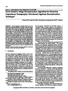
G. Comparisons We evaluated the above approximations for a wide variety of simulated and real fieldmaps. We summarize here one representative comparison, using the brain fieldmap shown in Fig. 1. This map, a brain slice near the ear canals, was acquired using standard delayed-echo field mapping methods on a GE 3T MR scanner [51]. Fig. 2 shows the histogram of this field map. For evaluation, we used ti ’s with 5 µs sampling for M = 3770, corresponding to a 18.855 ms readout time. This time is typical for one-shot spiral trajectories on our 3T GE scanner for 64 × 64 brain scans with a 22 cm FOV. We compared four approximations: (i) the SVD approach of §III-D using the histogram approximation (20) with K = 40 bins; (ii) the time-segmentation (TS) approach of §III-F with the WLS criterion (21); (iii) the frequency segmentation (FS) method of §III-E using the LS-optimal interpolators (19). For FS, we found that uniformly spaced zˇl values worked well only for a simple fieldmap that varied linearly over space, which has a uniform field histogram (results not shown). As an alternative, we applied the Lloyd-Max algorithm from scalar quantizer design to choose the frequency samples from the fieldmap histograms. This reduced error in all cases. Fig. 3 shows the normalized root mean-squared error (NRMSE), defined by N1 |||E − BC|||Frob (see (18)), as a function of L for the fieldmap shown in Fig. 1, for all four approximations. Naturally, as the number of approximation terms L increases, the error decreases. In all cases, for any given L the SVD approach has the minimum error. However, the TS approximation has only slightly larger error. In fact, to achieve a NRMSE less than 1%, both the SVD and the TS methods require L = 6 for this fieldmap. From these representative results and others not shown, we conclude that TS approximations, when optimized per §III-F, provide the most attractive tradeoff between accuracy and ease of computation. This conclusion is fortuitous since the Toeplitz approach described in §IV is most efficient when implemented with TS approximations. IV. T OEPLITZ APPROACH Now we turn to computing the “Toeplitz approach” (13) efficiently. Under the model (9), the matrix T in (13) has the

5

following elements: Fieldmap: Brain 1

Tkj

120

=

[A0 A]kj =

M X

a∗ik aij

i=1

100

=

80

i=1

2

∗

|Pi | e−(zk +zj )ti e−ı2π~νi ·(~rj −~rk ) .

(22)

In the usual case where the voxel centers ~rj are spaced equally, this matrix would be Toeplitz3 in the absence of relaxation effects and off-resonance effects, i.e., when z(~r) = 0. In the presence of such effects, T is not Toeplitz due ∗ to the problematic term e−(zk +zj )ti . So we must introduce approximations to develop fast methods for computing the matrix-vector product T x required in the gradient calculation (13). Two possible approaches are described next.

Hz

60 40

M X

20 0 −20 64 1

64

A. O(L2 ) approach One approach is to separate the problematic exponential first, and then make approximations as follows: !∗ L L X X ∗ ∗ −(zk −zk +zj )ti ti −zj ti bil clj , e ≈ bil0 cl0 k =e e

Brain field map ω(~ r ) /2π.

Fig. 1.

Fieldmap histogram: Brain 100

l0 =1

i.e., to invoke approximations of the form (14) twice. Substituting into (22) and rearranging leads to the following:

80

T ≈

60

[T

l0 ,l

]kj =

20

Dl00 Tl0 ,l Dl ,

(23)

l0 =1 l=1

M X i=1

0 −50

0

50 Hz

100

Histogram of the fieldmap shown in Fig. 1. Brain

0

B. O(L) approach To reduce computation, we would like to use an approximation for the problematic exponential term that will allow us to “separate” the zk∗ +zj term in (22) after making the approximation. Of the various approximation methods described in §III, only the time segmentation approach appears to have the desired property. (Fortunately the time segmentation approach is also sufficiently accurate, as shown in §III-G.) Substituting the approximation (16) (with z¯ = 0) into (22) yields the following approximation to the elements of T : " L # M X X ∗ 2 −(zk +zj )tˇl Tkj ≈ |Pi | bil e e−ı2π~νi ·(~rj −~rk )

FS uniform FS quantized TS uniform SVD

−1

10

−2

10

−3

10

−4

10

2

|Pi | b∗il0 bil e−ı2π~νi ·(~rj −~rk ) .

Each matrix Tl0 ,l is Toeplitz, so we can multiply this approximation to T by a vector x using L2 pairs of FFTs [47]. An advantage of this approach is that one can use the B and C matrices corresponding to any exponential approximation (14). But a significant disadvantage is that it requires O(L2 ) computation.

10

NRMSE

L L X X

where Dl = diag{clj } and

40

Fig. 2.

l=1

i=1

2

4

6

8

10

L

Fig. 3. Normalized RMS error for approximations to the exponentials e for the field map shown in Fig. 1.

= −zj ti

,

L X

l=1

∗ˇ

ˇ

e−zk tl [Tl ]kj e−zj tl ,

l=1

3 For simplicity, we say “Toeplitz” rather than “block Toeplitz with Toeplitz blocks” [47].

(24)

6

where the element of each matrix Tl are defined by [Tl ]kj =

M X i=1

In matrix form,

2

|Pi | bil e−ı2π~νi ·(~rj −~rk ) .

T ≈

L X

Dl0 Tl Dl ,

(25)

(26)

l=1

o n where Dl = diag e−zj tˇl . Each matrix Tl is Toeplitz, so one can multiply Tl by a vector efficiently using a pair of FFTs [47]. These FFTs use the first row of Tl , which we precompute prior to iterating by a pair of NUFFT calls. Each Dl matrix is diagonal, so multiplying with it is trivial. Thus, to compute T x (approximately) requires L pairs of FFTs, for an operation count of O(LN log N ). In contrast, the NUFFT approach that uses the gradient expression in (12) with an approximation like (15) requires L pairs of NUFFTs, which is more computation due to interpolations [46]. A subtle but key issue in using (24) is choosing the interpolators bil . If the rate map zj contains frequency offsets ∗ in the range νmin to νmax , then the term e−(zk +zj )t will contain frequency offsets in the range −(νmax − νmin ) to νmax − νmin . In other words, its “bandwidth” is twice as wide as the bandwidth of e−zj t . So we have found that it can be necessary to use larger values of L for the Toeplitz approximation (24) than for the NUFFT approximation (15). Nevertheless, by avoiding DFT interpolations, the Toeplitz approach is still faster than the NUFFT approach. For (25) to be accurate, we would like to choose B to ∗ provide a LS approximation to terms of the form e−(zk +zj )ti . For a fieldmap with a given histogram {hk }, the histogram of zk∗ + zj is given by the auto-correlation function of hk . So to design B for the Toeplitz approach, we first find the fieldmap histogram, then compute the auto-correlation function of that histogram, and then apply the WLS criterion (21) using that auto-correlated histogram. We found that this approach provided much improved accuracy relative to using (21) with the original histogram. Furthermore, because “autocorrelated” histograms are symmetric about zero, the resulting B matrix is real valued, saving computation in precomputing the Toeplitz kernels in (25). We summarize all of the required steps as follows. Fig. 4 illustrates the data flow4 . CG-Toeplitz Algorithm • Determine the relaxation map and/or the field map to form the rate map z(~r) in (4). • Compute the histogram of that rate map, and then the autocorrelation function of that histogram. • Using that auto-correlated histogram, use (21) and (16) to compute the interpolators B and the coefficients C using the LS time-segmentation method of §III-F. • Precompute b = A0 y using the combination of temporal interpolation and NUFFT methods described in [21], [46]. Since this need only be done once, rather than each iteration, it can be done with a high accuracy approximation. 4 Software available on web site http://www.eecs.umich.edu/∼fessler.

• Precompute the first row of Tl for l = 1, . . . , L using (25), in preparation for using a 2× over-sampled FFT to perform the operation of matrix-vector multiplication by Tl [47]. This requires L pairs of NUFFT calls. • Using (26) to compute T x approximately for the gradient expression (13), apply a gradient-based optimization ˆ method such as the CG algorithm (e.g., [21]) to find x iteratively. Field Map (Optional)

B

Design basis and coefficients

Compute FFT of Toeplitz matrix row

Relax Map (Optional)

C MR k−space Measured Data

Fig. 4.

y

Tl

Gradient−based Optimization

Image Display

Block diagram of MR image reconstruction data flow.

V. S IMULATION We compared four methods for field-corrected MR image reconstruction: (i) the conjugate-phase reconstruction method [5] using Voronoi-based density compensation factors [52] and the LS-optimal time-segmentation approximation described in §III-F, (ii) the CG-NUFFT method based on the gradient expression (12), using the time-segmentation approximation described in §III-F [21], (iii) the CG-Toeplitz method based on the gradient expression (13) using the O(L) approximation described in §IV, and (iv) for completeness, the conjugatephase method without field correction. For the CG methods we used quadratic regularization with a small regularization parameter, chosen such that the FWHM of the PSF was about 1.36 pixels. For simplicity we initialized the CG algorithms with x = 0. To evaluate the methods quantitatively, we performed simulations using the brain fieldmap shown in Fig. 1, and the synthetic image x shown in Fig. 5. We evaluated the reconstruction methods using a spiral trajectory containing 3770 points with a sampling time of 5 µs, so the data acquisition time was 18.855 ms. This spiral trajectory is used routinely on our GE 3T MR system. To generate the (noiseless) simulated ¯ we used the exact system matrix (10). data y, For all methods, we estimated only the 2936 pixels within the elliptical region of interest shown in Fig. 5. For reconstruction, we used NUFFTs with 2× over-sampling and J = 6, which we have found previously to be sufficiently accurate. Fig. 6 shows the NRMS error as a function of iteration, ˆ − xtrue k / kxtrue k · 100%, for the values of L defined as kx listed. Larger values of L did not reduce the error further. Since there was no noise in the simulated k-space data, the lower limit on NRMS error is a function of the (modest) regularization used and the inherent NUFFT approximations. For these values of L (or larger) the CG algorithm essentially converged by 15 iterations.

7

Image and support 2.5

1

64

0 1

64

Fig. 5. True image x used in simulations. Only pixels within the outer elliptical region were reconstructed.

Toeplitz L=6 Toeplitz L=7 NUFFT L=5 NUFFT L=6

30 25 % NRMSE

Fig. 7 shows the NRMS error as a function of L. To achieve the same accuracy, the CG-Toeplitz approach requires L to be slightly larger than for CG-NUFFT. The RMS error of the CP method changes relatively little for L > 1, apparently because that error is dominated by imperfect density compensation for the spiral trajectory. We separately examined a Cartesian trajectory (results not shown), where density compensation is moot, and in that case the NRMS error decreased monotonically in L until reaching a minimum value of 14% at L = 6. Fig. 8 shows the reconstructed images. Based on the results in Fig. 7, we used L = 6 for the conjugate phase and CGNUFFT approaches, and L = 8 for the CG-Toeplitz approach. Table I compares the CPU time of the various reconstruction methods (using M ATLAB’s cputime on a Dell 650n with 3.06GHz Xeon CPU). For the CG methods, the times are for 15 iterations, which is adequate based on Fig. 6. The total times shown in the table include the time required to “precompute” B, C, etc. The Toeplitz approach shows significant acceleration. In M ATLAB, for the same L the Toeplitz approach runs several times faster per iteration than the NUFFT approach, because it avoids the NUFFT interpolations. The Toeplitz approach requires a slightly larger value for L and requires precomputing the kernels of the Tl terms, but despite this “overhead” the overall compute time is still reduced significantly. To investigate whether the approximations would increase sensitivity to noise, we added several different levels of pseudo-random white complex gaussian noise to y¯ and repeated the reconstructions. Table I shows that the noise properties of the CG-NUFFT and CG-Toeplitz approach are indistinguishable, because the chosen L values ensure that approximation error is negligible relative to estimation error.

20 15 10 5 0 0

5

10

15

Iteration ˆ versus iteration for the two CG reconstruction methods Fig. 6. NRMSE of x for the spiral trajectory.

30 CP CG with NUFFT CG with Toeplitz

25 % NRMSE

VI. S UMMARY This paper has described a new CG-Toeplitz method for field-corrected MR image reconstruction using the approximations (26). Simulation results show that this proposed method is as accurate as the previously proposed CG-NUFFT method [21] but is considerably faster. The CG-Toeplitz approach is also better suited to fast hardware implementation since only FFTs are required during the iterations, eliminating the frequency domain interpolations required by the CG-NUFFT approach. We believe the CG-Toeplitz approach is the method of choice for iterative field-corrected MR image reconstruction. The improved image quality in regions with severe field inhomogeneity may enable detection of brain activation even in regions near air/tissue interfaces. An alternative CG approach has recently proposed by Barnet et al. [53]. That approach involves expressions of the form AA0 , which is never Toeplitz, even when the rate map is zero, so it cannot benefit from the accelerations proposed here. Furthermore, it is limited to the special case of quadratic regularization with an invertible Hessian, whereas the gradientbased approach that uses (12) or (13) can accommodate even non-quadratic regularization methods, e.g., [54]. There are several opportunities to extend this work. • When z(~r) = 0, the matrix T in (22) is Toeplitz, and good circulant preconditioners are available [47]. When z(~r) 6=

20 15 10 5 0

2

4

6

8

10

L ˆ versus approximation order L for the three fieldFig. 7. NRMSE of x corrected reconstruction methods for the spiral trajectory.

8

Method Conj. Phase CG-NUFFT CG-Toeplitz

L 6 6 8

B,C 0.4 0.4 0.4

Precomputation A0 Dy b = A0 y 0.2 0.2

Tl

15 iter

0.6

5.0 1.3

Total Time 0.6 5.4 2.5

∞ 30.7 5.6 5.5

NRMS % vs SNR 50 dB 40 dB 30 dB 37.3 46.5 65.3 16.7 26.5 43.0 16.7 26.4 42.9

20 dB 99.9 70.4 70.4

TABLE I CPU TIMES ( SECONDS ), INCLUDING PRECOMPUTATION TIMES , AND NRMS ERROR (%) FOR THREE FIELD - CORRECTED MR IMAGE RECONSTRUCTION METHODS . T HE PROPOSED CG-T OEPLITZ APPROACH IS FASTER THAN CG-NUFFT YET EQUALLY ACCURATE .

Uncorrected Conj. Phase, L=6

methods may tolerate smaller over-sampling factors [41]. Whether the Toeplitz approach could also tolerate reduced over-sampling requires further investigation, particularly in the presence of field inhomogeneity. • For the methods described here, we separated the problems of designing the “temporal” interpolators B and C and of designing the interpolators that are used in the frequency domain for the NUFFT operation. Whether one could design both interpolators simultaneously to improve accuracy (or reduce computation) is an interesting challenge. ACKNOWLEDGEMENT We thank Dave Neuhoff for recommending [50]. R EFERENCES

CG−NUFFT L=6

CG−Toeplitz L=8

0 Fig. 8.

2.5 Reconstructed images for the spiral trajectory.

0, then T is approximately the “weighted sum” of Toeplitz matrices in (26). An open question for future work is how to precondition this sum effectively; preconditioners have been developed for other shift-variant problems [47], [55]. • The model (6) assumes that the rate map is constant over each voxel. To compensate for within-voxel field gradients, one can use smaller voxels [44]. This increases computation, so an interesting challenge is to try to account for field gradients with less computation. • For echo-planar imaging (EPI), the primary blur in the readout direction. This affects the properties of the Tl matrices, and it may be possible to further reduce computation. • For both the NUFFT and Toeplitz methods investigated here, we used FFTs with 2× over-sampling in each dimension. In the absence of field inhomogeneity, NUFFT-type

[1] E. M. Haacke, R. W. Brown, M. R. Thompson, and R. Venkatesan, Magnetic resonance imaging: Physical principles and sequence design. New York: Wiley, 1999. [2] S. Ogawa, R. S. Menon, D. W. Tank, S. G. Kim, H. Merkle, J. M. Ellermann, and K. Ugurbil, “Functional brain mapping by blood oxygenation level-dependent contrast magnetic resonance imaging. A comparison of signal characteristics with a biophysical model,” Biophys. J., vol. 64, no. 3, pp. 803–12, Mar. 1993. [3] K. Sekihara, S. Matsui, and H. Kohno, “NMR imaging for magnets with large nonuniformities,” IEEE Tr. Med. Imag., vol. 4, no. 4, pp. 193–9, Dec. 1985. [4] E. Yudilevich and H. Stark, “Spiral sampling in magnetic resonance imaging - the effect of inhomogeneities,” IEEE Tr. Med. Imag., vol. 6, no. 4, Dec. 1987. [5] D. C. Noll, C. H. Meyer, J. M. Pauly, D. G. Nishimura, and A. Macovski, “A homogeneity correction method for magnetic resonance imaging with time-varying gradients,” IEEE Tr. Med. Imag., vol. 10, no. 4, pp. 629–37, Dec. 1991. [6] D. C. Noll, J. M. Pauly, C. H. Meyer, D. G. Nishimura, and A. Macovski, “Deblurring for non-2D Fourier transform magnetic resonance imaging,” Mag. Res. Med., vol. 25, pp. 319–33, 1992. [7] H. Chang and J. M. Fitzpatrick, “A technique for accurate magnetic resonance imaging in the presence of field inhomogeneities,” IEEE Tr. Med. Imag., vol. 11, no. 3, pp. 319–29, Sept. 1992. [8] T. S. Sumanaweera, G. H. Glover, T. O. Binford, and J. R. Adler, “MR susceptibility misregistration correction,” IEEE Tr. Med. Imag., vol. 12, no. 2, pp. 251–9, June 1993. [9] P. Jezzard and R. S. Balaban, “Correction for geometric distortion in echo planar images from B0 field variations,” Mag. Res. Med., vol. 34, no. 1, pp. 65–73, July 1995. [10] Y. M. Kadah and X. Hu, “Simulated phase evolution rewinding (SPHERE): A technique for reducing B0 inhomogeneity effects in MR images,” Mag. Res. Med., vol. 38, pp. 615–27, 1997. [11] ——, “Algebraic reconstruction for magnetic resonance imaging under B0 inhomogeneity,” IEEE Tr. Med. Imag., vol. 17, no. 3, pp. 362–70, June 1998. [12] T. B. Harshbarger and D. B. Twieg, “Iterative reconstruction of singleshot spiral MRI with off-resonance,” IEEE Tr. Med. Imag., vol. 18, no. 3, pp. 196–205, Mar. 1999. [13] H. Schomberg, “Off-resonance correction of MR images,” IEEE Tr. Med. Imag., vol. 18, no. 6, pp. 481–95, June 1999.

9

[14] J. Kybic, P. Thevenaz, A. Nirkko, and M. Unser, “Unwarping of unidirectionally distorted EPI images,” IEEE Tr. Med. Imag., vol. 19, no. 2, pp. 80–93, Feb. 2000. [15] P. Munger, G. R. Crelier, T. M. Peters, and G. B. Pike, “An inverse problem approach to the correction of distortion in EPI images,” IEEE Tr. Med. Imag., vol. 19, no. 7, pp. 681–9, July 2000. [16] K. S. Nayak and D. G. Nishimura, “Automatic field map generation and off-resonance correction for projection reconstruction imaging,” Mag. Res. Med., vol. 43, no. 1, pp. 151–4, Jan. 2000. [17] K. S. Nayak, C.-M. Tsai, C. H. Meyer, and D. G. Nishimura, “Efficient off-resonance correction for spiral imaging,” Mag. Res. Med., vol. 45, no. 3, pp. 521–4, Mar. 2001. [18] J. A. Akel, M. Rosenblitt, and P. Irarrazaval, “Off-resonance correction using an estimated linear time map,” Mag. Res. Im., vol. 20, no. 2, pp. 189–98, Feb. 2002. [19] R. Deichmann, O. Josephs, C. Hutton, D. R. Corfield, and R. Turner, “Compensation of susceptibility-induced BOLD sensitivity losses in echo-planar fMRI imaging,” NeuroImage, vol. 15, no. 1, pp. 120–35, Jan. 2002. [20] H. Moriguchi, B. M. Dale, J. S. Lewin, and J. L. Duerk, “Block regional off-resonance correction (BRORC): A fast and effective deblurring method for spiral imaging,” Mag. Res. Med., vol. 50, no. 3, pp. 643–8, Sept. 2003. [21] B. P. Sutton, D. C. Noll, and J. A. Fessler, “Fast, iterative image reconstruction for MRI in the presence of field inhomogeneities,” IEEE Tr. Med. Imag., vol. 22, no. 2, pp. 178–88, Feb. 2003. [22] D. C. Noll, J. A. Fessler, and B. P. Sutton, “Conjugate phase MRI reconstruction with spatially variant sample density correction,” IEEE Tr. Med. Imag., vol. 24, no. 3, Mar. 2005, to appear. [23] B. P. Sutton, D. Noll, and J. A. Fessler, “Simultaneous estimation of image and inhomogeneity field map,” in ISMRM Minimum Data Acquisition Workshop, 2001, pp. 15–8. [24] B. P. Sutton, J. A. Fessler, and D. C. Noll, “Field-corrected imaging using joint estimation of image and field map,” in Proc. Intl. Soc. Mag. Res. Med., 2002, p. 737. [25] B. P. Sutton, D. C. Noll, and J. A. Fessler, “Dynamic field map estimation using a spiral-in / spiral-out acquisition,” Mag. Res. Med., vol. 51, no. 6, pp. 1194–204, June 2004. [26] S. Lee, S. J. Peltier, J. A. Fessler, and D. Noll, “Estimation of R2∗ using extended rosette acquisition,” in Hum. Brain Map., 2002, pp. 151–2, in NeuroImage 16(2 S1):151-2, 2002. [27] V. T. Olafsson, D. C. Noll, and J. A. Fessler, “New approach for estimating ∆R2∗ in fMRI,” in Proc. Intl. Soc. Mag. Res. Med., 2003, p. 132. [28] O. Speck and J. Hennig, “Functional imaging by I0 and T2∗ -parameter mapping using multi-image EPI,” Mag. Res. Med., vol. 40, pp. 243–8, 1998. [29] S. Lee, J. A. Fessler, and D. Noll, “A simultaneous estimation of field inhomogeneity and R2* maps using extended rosette trajectory,” in Proc. Intl. Soc. Mag. Res. Med., 2002, p. 2327. [30] B. P. Sutton, S. J. Peltier, J. A. Fessler, and D. C. Noll, “Simultaneous estimation of I0 , R2∗ , and field map using a multi-echo spiral acquisition,” in Proc. Intl. Soc. Mag. Res. Med., 2002, p. 1323. [31] S. J. Peltier, B. P. Sutton, J. A. Fessler, and D. C. Noll, “Simultaneous estimation of I0 , R2∗ , and field map using a multi-echo spiral acquisition,” in Hum. Brain Map., 2002, pp. 95–6, in NeuroImage 16(2 S1):956, 2002. [32] H. Eggers, T. Schaeffter, B. Aldefeld, and P. Boesiger, “Combined ∆B0 and T2∗ correction for radial multi-gradient-echo imaging,” in Proc. Intl. Soc. Mag. Res. Med., 2003, p. 478. [33] D. B. Twieg, “Parsing local signal evolution directly from a single-shot MRI signal: A new approach for fMRI,” Mag. Res. Med., vol. 50, no. 5, pp. 1043–52, Nov. 2003. [34] S. Lee, D. Noll, and J. A. Fessler, “EXTended Rosette ACquisition Technique (EXTRACT): a dynamic R2* mapping method using extended rosette trajectory,” in Proc. Intl. Soc. Mag. Res. Med., 2004, p. 2128. [35] V. Olafsson, J. A. Fessler, and D. C. Noll, “Dynamic update of R2* and field map in fMRI,” in Proc. Intl. Soc. Mag. Res. Med., 2004, p. 45. [36] B. P. Sutton, J. A. Fessler, and D. Noll, “Iterative MR image reconstruction using sensitivity and inhomogeneity field maps,” in Proc. Intl. Soc. Mag. Res. Med., 2001, p. 771. [37] D. C. Noll, “Reconstruction techniques for magnetic resonance imaging,” Ph.D. dissertation, Stanford, CA, 1991. [38] K. P. Pruessmann, M. Weiger, P. B¨ornert, and P. Boesiger, “Advances in sensitivity encoding with arbitrary k-space trajectories,” Mag. Res. Med., vol. 46, no. 4, pp. 638–51, Oct. 2001.

[39] K. Gr¨ochenig and T. Strohmer, “Numerical and theoretical aspects of non-uniform sampling of band-limited images,” in Nonuniform Sampling: Theory and Practice, F. Marvasti, Ed. New York: Kluwer, 2001, pp. 283–324. [40] F. Wajer and K. P. Pruessmann, “Major speedup of reconstruction for sensitivity encoding with arbitrary trajectories,” in Proc. Intl. Soc. Mag. Res. Med., 2001, p. 767. [41] H. Eggers and P. B. P. B., “Comparison of gridding- and convolutionbased iterative reconstruction algorithms for sensitivity-encoded noncartesian acquisitions,” in Proc. Intl. Soc. Mag. Res. Med., 2002, p. 743. [42] R. M. Lewitt and S. Matej, “Overview of methods for image reconstruction from projections in emission computed tomography,” Proc. IEEE, vol. 91, no. 9, pp. 1588–611, Oct. 2003. [43] R. Van de Walle, H. H. Barrett, K. J. Myers, M. I. Altbach, B. Desplanques, A. F. Gmitro, J. Cornelis, and I. Lemahieu, “Reconstruction of MR images from data acquired on a general non-regular grid by pseudoinverse calculation,” IEEE Tr. Med. Imag., vol. 19, no. 12, pp. 1160–7, Dec. 2000. [44] B. P. Sutton, D. C. Noll, and J. A. Fessler, “Compensating for withinvoxel susceptibility gradients in BOLD fMRI,” in Proc. Intl. Soc. Mag. Res. Med., 2004, p. 349. [45] B. P. Sutton, “Physics-based reconstruction of magnetic resonance images,” Ph.D. dissertation, Univ. of Michigan, Ann Arbor, MI, 481092122, Ann Arbor, MI., 2003. [46] J. A. Fessler and B. P. Sutton, “Nonuniform fast Fourier transforms using min-max interpolation,” IEEE Tr. Sig. Proc., vol. 51, no. 2, pp. 560–74, Feb. 2003. [47] R. H. Chan and M. K. Ng, “Conjugate gradient methods for Toeplitz systems,” SIAM Review, vol. 38, no. 3, pp. 427–82, Sept. 1996. [48] P. Irarrazabal, C. H. Meyer, D. G. Nishimura, and A. Macovski, “Inhomogeneity correction using an estimated linear field map,” Mag. Res. Med., vol. 35, pp. 278–82, 1996. [49] L.-C. Man, J. M. Pauly, and A. Macovski, “Multifrequency interpolation for fast off-resonance correction,” Mag. Res. Med., vol. 37, pp. 785–92, 1997. [50] A. Gersho, “Asymptotically optimal block quantization,” IEEE Tr. Info. Theory, vol. 25, no. 4, pp. 373–380, July 1979. [51] M. R. Willcott, G. L. Mee, and J. P. Chesick, “Magnetic field mapping in NMR imaging,” Mag. Res. Med., vol. 5, no. 4, pp. 301–6, 1987. [52] H. Schomberg and J. Timmer, “The gridding method for image reconstruction by Fourier transformation,” IEEE Tr. Med. Imag., vol. 14, no. 3, pp. 596–607, Sept. 1995. [53] C. Barnet, J. Tsao, and K. P. Pruessmann, “Efficient iterative reconstruction for MRI in strongly inhomogeneous B0 ,” in Proc. Intl. Soc. Mag. Res. Med., 2004, p. 347. [54] J. A. Fessler and D. C. Noll, “Iterative image reconstruction in MRI with separate magnitude and phase regularization,” in Proc. IEEE Intl. Symp. Biomedical Imaging, 2004, pp. 209–12. [55] J. A. Fessler and S. D. Booth, “Conjugate-gradient preconditioning methods for shift-variant PET image reconstruction,” IEEE Tr. Im. Proc., vol. 8, no. 5, pp. 688–99, May 1999.

10

Jeff Fessler earned a Ph.D. in electrical engineering in 1990 from Stanford University. He has since worked at the University of Michigan, first as a DoE Alexander Hollaender post-doctoral fellow and then as an Assistant Professor in the Division of Nuclear Medicine. Since 1995 he has been with the EECS Department, the BME Department, and the Radiology Department. His research interests are in statistical aspects of imaging problems, and he has supervised doctoral research in PET, SPECT, X-ray CT, MRI, and optical imaging.

L IST OF TABLES I

4 5

6 7

Valur Olafsson (SM’05) received the B.S. degree in electrical engineering from the University of Iceland, Reykjavik, Iceland, in 2000, the M.S. degree in electrical engineering from the University of Michigan, Ann Arbor, MI, in 2003, where he is currently a doctoral student. His current research interests are in iterative MR image reconstruction methods.

Hugo Shi received a BS in EECS from the University of California at Berkeley in 2003. He is currently a second year graduate student at the University of Michigan studying EE systems, with an emphasis in Medical Image Processing. His current research interests include regularization design for statistical image reconstruction from 3D PET scans.

Since 1998, Dr. Noll has been Associate Professor of Biomedical Engineering and Radiology and CoDirector of the Functional MRI Laboratory at the University of Michigan, Ann Arbor. From 19911998, Dr. Noll was with the Department of Radiology at the University of Pittsburgh. His expertise is in magnetic resonance image acquisition, reconstruction and processing with a focus on functional brain imaging. Dr. Noll received his M.S. and Ph.D. in electrical engineering from Stanford University, Stanford, CA in 1986 and 1991, respectively and received his B.S. in electrical engineering from Bucknell University, Lewisburg, PA in 1985. He is a member of the IEEE, the International Society for Magnetic Resonance in Medicine and is fellow of the American Institute for Medical and Biological Engineering.

8

L IST OF F IGURES 1 2 3

Sangwoo Lee (S’00) was born in Seoul, Korea in 1973. He received the B.S.E. degree in electrical engineering from Seoul National University in 1996, and the M.S.E. degree from the Department of Electrical Engineering and Computer Science at the University of Michigan in 2001, where he is currently pursuing the PhD degree in signal processing. His research interests include statistical iterative MR (Magnetic Resonance) image reconstruction and MR pulse sequence design.

CPU times (seconds), including precomputation times, and NRMS error (%) for three fieldcorrected MR image reconstruction methods. The proposed CG-Toeplitz approach is faster than CG-NUFFT yet equally accurate. . . . . . . . .

8

Brain field map ω(~r) /2π. . . . . . . . . . . . . Histogram of the fieldmap shown in Fig. 1. . . . Normalized RMS error for approximations to the exponentials e−zj ti , for the field map shown in Fig. 1. . . . . . . . . . . . . . . . . . . . . . . . Block diagram of MR image reconstruction data flow. . . . . . . . . . . . . . . . . . . . . . . . . True image x used in simulations. Only pixels within the outer elliptical region were reconstructed. . . . . . . . . . . . . . . . . . . . . . . ˆ versus iteration for the two CG NRMSE of x reconstruction methods for the spiral trajectory. . ˆ versus approximation order L for NRMSE of x the three field-corrected reconstruction methods for the spiral trajectory. . . . . . . . . . . . . . . Reconstructed images for the spiral trajectory. . .

5 5

5 6

7 7

7 8