Topological fault-tolerance in cluster state quantum computation

Topological fault-tolerance in cluster state quantum computation R. Raussendorf1 , J. Harrington2 and K. Goyal3 1

Perimeter Institute for Theoretical Physics, Waterloo, ON, M6P 1N8, Canada Applied Modern Physics, MS D454, Los Alamos National Laboratory, Los Alamos, NM 87545, USA 3 Institute for Quantum Information, California Institute of Technology, Pasadena, CA 91125, USA

arXiv:quant-ph/0703143v1 16 Mar 2007

2

February 1, 2008 Abstract We describe a fault-tolerant version of the one-way quantum computer using a cluster state in three spatial dimensions. Topologically protected quantum gates are realized by choosing appropriate boundary conditions on the cluster. We provide equivalence transformations for these boundary conditions that can be used to simplify fault-tolerant circuits and to derive circuit identities in a topological manner. The spatial dimensionality of the scheme can be reduced to two by converting one spatial axis of the cluster into time. The error threshold is 0.75% for each source in an error model with preparation, gate, storage and measurement errors. The operational overhead is poly-logarithmic in the circuit size.

1

Introduction

The threshold theorem for fault-tolerant quantum computation [1, 2, 3, 4] has established the fact that large quantum computations can be performed with arbitrary accuracy, provided that the error level of the elementary components of the quantum computer is below a certain threshold. It now becomes important to devise methods for error correction which yield a high threshold, are robust against variations of the error model, and can be implemented with small operational overhead. An additional desideratum is a simple architecture for the quantum computer, such as requiring no long-range interaction. The one-way quantum computer provides a method to do this [5, 6], which we describe in detail below. We obtain an error threshold estimate of 0.75% for each source in an error model with preparation, gate, storage and measurement errors, with a poly-logarithmic multiplicative overhead in the circuit size Ω (∼ ln3 Ω). It shall be noted that we achieve this threshold in a 2-dimensional geometry, only requiring nearest-neighbor translation-invariant Ising interaction. This is relevant for experimental realizations based on matter qubits such as cold atoms in optical lattices [7, 8] and two-dimensional ion traps [9], or stationary qubits in quantum dot systems [10] and arrays of superconducting qubits [11]. Geometric constraints are no major concern for fault-tolerant quantum computation with photonic qubits [12, 13]. The highest known threshold estimate, for a setting without geometric constrains, is 3 × 10−2 [14]. Fault-tolerance is more difficult to achieve in architectures where each qubit can only interact with other qubits in its immediate neighborhood. A recent fault-tolerance threshold for a twodimensional lattice of qubits with only local and nearest-neighbor gates is 1.9 × 10−5 [15]. We note that since the initial work of [16] a number of distinct approaches to topological fault-tolerance emerging in lattice systems are being pursued; See [17, 18, 19, 20]. The key element of our method is based on topological tools that become available when the dimensionality of the cluster is increased from two to three. In 3D, we combine the universality already found in 2D cluster states [21] with the topological error-correcting capability of Kitaev’s 1

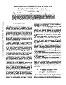
Figure 1: Topologically protected gates.

toric code [16]. Then, a one-dimensional sub-structure of the cluster is “carved out” by performing local Z-measurements. This leaves us with a non-trivial cluster topology in which a fault-tolerant quantum circuit is embedded. Fig. 1 displays topologically protected gates that can be constructed in this manner. This paper is organized as follows. In the remainder of this section we introduce the necessary terminology for discussion of the fault-tolerant QCC . In Section 2 we answer the question of “Why can we perform non-abelian gates with surface codes?” and describe topological transformation rules on the cluster. We subsequently use these rules to simplify topological circuits. In Section 3 we complete the universal set of gates. In Section 4 we describe the mapping from a 3D cluster state to a two-dimensional physical system plus time. Sections 5 and 6 address the fault-tolerance threshold and overhead, respectively. We conclude with a summary and outlook in Section 7. Before we can start our discussion of the fault-tolerance properties of the QCC , we need to introduce some necessary notation. This has been done before in [5, 6]. We include a short introduction here to make our presentation self-contained. Consider a cluster state |φiL on a lattice L with elementary cell as displayed in Fig. 2a. Qubits are located at the center of faces and edges of L. The lattice L is subdivided into three regions V , D and S. Each region has its purpose, shape and specific measurement basis for its qubits. The qubits in V are measured in the√X-basis, the qubits in D in the Z-basis, and the qubits in S in either of the eigenbases (X ± Y )/ 2. V fills up most of the cluster. D is composed of thick line-like structures, named defects. S is composed of well-separated qubit locations interspersed among the defects. As described in greater detail below, the cluster region V provides topological error correction, while regions D and S specify the Clifford and non-Clifford parts of a quantum algorithm, respectively. We can break up this measurement pattern into gate simulations by establishing the following correspondence: quantum gates ↔ quantum correlations ↔ surfaces. The first part of this correspondence has been established in [22]. For the second part homology comes into play. The correlations of |φiL , i.e., the stabilizers, can be identified with 2-chains (surfaces) in L, while errors map to 1-chains (lines). Homological equivalence of the chains implies physical equivalence of the corresponding operators [5]. This correspondence is key to the presented scheme. Gates are specified by a set of surfaces with input and output boundaries, and syndrome measurements correspond to closed surfaces (having no boundary). L is regarded as a chain complex, L = {C3 , C2 , C1 , C0 }. It has a dual L = {C 3 , C 2 , C 1 , C 0 } whose cubes c3 ∈ C 3 map to sites c0 ∈ C0 of L, whose faces c2 ∈ C 2 map to edges c1 ∈ C1 of L, etc. The chains have coefficients in Z2 . One may switch back and forth between L and L by a duality transformation ∗ ( ). L and L are each equipped with a boundary map ∂, where ∂ ◦ ∂ = 0. Operators may be associated with chains as follows. Suppose that for each qubit location a in a chain c,Qa ∈ {c}, there exists an operator Σa , and [Σa , Σb ] = 0 for all a, b ∈ {c}. Then, we define Σ(c) := a∈{c} Σa . Cluster state correlations (i.e. stabilizers) are associated with 2-chains. For 2

the considered lattice, all elements in the cluster state stabilizer take the form K(c2 )K(c2 ) with c2 ∈ C2 , c2 ∈ C 2 , and (1) K(c2 ) = X(c2 )Z(∂c2 ), K(c2 ) = X(c2 )Z(∂c2 ). Only those stabilizer elements compatible with the local measurement scheme are useful for information processing. In particular, they need to commute with the measurements in V and D, [K(c2 )K(c2 ), Xa ] = 0, [K(c2 )K(c2 ), Zb ] = 0,

a ∈ V, b ∈ D.

(2)

Due to the presence of a primal lattice L and a dual lattice L, it is convenient to subdivide the sets V and D into primal and dual subsets. Specifically, V = Vp ∪ Vd , with Vp ⊂ {C2 }, Vd ⊂ {C 2 }, and D = Dp ∪ Dd , with Dp ⊂ {C1 }, Dd ⊂ {C 1 }. With these notions introduced the compatibility condition (2) may be expressed directly in terms of the chains c2 and c2 . If K(c2 ) and K(c2 ) have support in V ∪ D only then Eq. (2) is equivalent to {∂c2 } ⊂ Dp , {∂c2 } ⊂ Dd .

(3)

The QCC and surface codes. We need to specify the encoding of logical qubits before explaining the encoded gates. For this purpose, let us single out one spatial direction on the cluster as ‘simulating time.’ The perpendicular 2D slices provide space for a quantum code. The code which fills this plane after the mapping of the three dimensional lattice L onto a 2+1 dimensional one is the surface code [23]. The number of qubits which can be encoded in such a code depends solely on the surface topology. Here we consider a plane with pairs of either electric or magnetic holes. See Fig. 2b. A magnetic hole is a plaquette f where the associated stabilizer generator S(f ) = Z(∂f ) is not enforced on the code space, and an electric hole is a site s where the associated stabilizer S+ (s) = X(∂ # s) is not enforced on the code space (“#” denotes the duality transformation in 2D). Each hole is the intersection of a defect strand with a constant-time slice. A pair of holes supports a qubit. For a pair of magnetic holes f, f ′ , the encoded spin flip operator m m is X = X(c1 ), with {∂c1 } = {# f, # f ′ }, and the encoded phase flip operator is Z = Z(c1 ), with c1 ∼ = ∂f or c1 ∼ = ∂f ′ . The operator Z(∂f + ∂f ′ ) is in the code stabilizer S, Z(∂f + ∂f ′ ) ∈ S.

(4)

e e For a pair of electric holes s, s′ we have X = X(c′1 ), with c′1 ∼ = ∂ # s, Z = Z(c1 ), with {∂c1 } = {s, s′ }, and X(∂ # s + ∂ # s′ ) ∈ S. (5)

The simplest gate. Here we illustrate the relation between quantum gates, quantum correlations and correlation surfaces (2-chains). We choose the simplest possible example: the identity gate. The identity operation is realized by two parallel strands of defect of the same type. We consider a block shaped cluster C ⊂ L for the support of the identity gate. One of the spatial directions on the cluster is singled out as ‘simulated time.’ The two perpendicular slices of the cluster at the ‘earliest’ and ‘latest’ times represent the code surfaces I and O for the encoded qubit, with I, O ⊂ {C1 } being an integer number of elementary cells apart. As before, we ask which cluster state correlations K(c2 ), K(c2 ) are compatible with the local measurements in C\(I ∪ O). With the additional regions I and O present, the condition (2) turns into {c2 } ⊂ Vp , {c2 } ⊂ Vd ∪ I ∪ O,

{∂c2 } ⊂ Dp ∪ I ∪ O, {∂c2 } ⊂ Dd . 3

(6)

Figure 2: Lattice definitions. a) Elementary cell of the cluster lattice L. 1-chains of L (dashed lines), and graph edges (solid lines). b) A pair of electric (“e”) or magnetic (“m”) holes in the code e/m e/m and X denote the encoded Pauli operators Z and plane each support an encoded qubit. Z X, respectively.

Figure 3: Correlation surfaces σ2 , σ 2 for the identity gate on a primal qubit.

Surfaces of primal correlations compatible with the local measurements in C\(I ∪ O) can stretch through the cluster region V and end in the primal defects and the input- and output regions. They cannot end in a dual defect. Surfaces of dual correlations can stretch through V , I and O, and end in dual defects. They cannot end in primal defects1 . We now consider the identity gate on the primal qubit, mediated by a pair of primal defects. The relevant primal and dual correlation surfaces are displayed in Fig. 3, and we denote these special surfaces by σ2 and σ 2 . Before the local measurement of the qubits in C\(I ∪ O) the cluster state |φiC obeys K(σ2 )|φiC = K(σ 2 )|φiC = |φiC . Note that K(σ2 )|I∪O = Z I ⊗Z O and K(σ 2 )|I∪O = X I ⊗X O . The “·” refers to encoding with the surface code displayed in Fig. 2. Thus, for the state |ψiI∪O after the measurements in C\(I ∪ O), Z I ⊗ Z O |ψiI∪O = ±|ψiI∪O and X I ⊗ X O |ψiI∪O = ±|ψiI∪O . This is the connection between surfaces (2-chains) and quantum correlations. The connection between quantum correlations and gate operation has already been established in Theorem 1 of [22], from which the identity gate follows. The other Clifford gates (or more precisely, CSS-gates) are derived in a similar manner, invoking more complicated correlation surfaces. 1 The asymmetry between primal and dual 2-chains in Eq. (6) arises because I and O are chosen subsets of C1 . Physically speaking, we choose the sub-cluster C such that it consists of intact cells of the primal lattice L at the front and back. The cells of the dual lattice L are then cut in half at the front and back of C.

4

2 2.1

Topological considerations Why can we perform non-abelian gates with surface codes?

A limitation of the surface code [16, 23] is that only an abelian group of gates can be implemented fault-tolerantly by braiding operations [16]. In the fault-tolerant QCC , arbitrary CNOT-gates can be performed which are non-commuting. Yet, the fault-tolerance of the QCC is based on surface codes. How does this fit together? The reason why we can do non-abelian gates with a surface code in the QCC is that we change the topology of the code surface with time. The preparation of a primal |0i state (dual |+i state) introduces a pair of primal (dual) holes into the code surface. The corresponding measurements remove pairs of holes. The emergence of non-abelian gates through changes in the surface topology can be easily verified in the circuit model. Consider first the monodromy of a primal and a dual hole as the means to entangle two qubits of opposite type, .

(7)

This operation does not change the topology of the code surface. It can be checked with the methods described in Section 1 that operation (7) acts as a CNOT on the two involved qubits. However, the primal qubit is always the target and the dual qubit the control. These gates are still abelian. We now supplement these unitary commuting gates with non-unitary operations, namely Xand Z-preparations and measurements. They are obviously non-commuting and change the surface topology (See Fig. 1b). Can we construct non-commuting unitary operations out of this gate set? To this end, we assemble preparations, measurements and the monodromy operation (7) to the topological circuit displayed in Fig. 4a. It is a deformed version of the gate in Fig. 1a. Also, it can be verified directly in the circuit model that it represents a CNOT-gate (c.f. Fig. 4b). The direction of the CNOT can now be chosen freely, and we obtain a non-abelian set of unitary gates. The situation is somewhat reminiscent of the “tilted interferometry approach” [25]. There, the change of a surface topology with time is used to upgrade topological quantum computation with Ising-anyons from non-universal to universal. In our case, the change is from abelian to non-abelian. As a final comment, the change of surface topology with ‘time’ appears as a discontinuous process. This is an artifact of the mapping from 3 spatial dimensions to 2 spatial dimensions plus time. In the 3D cluster picture there is no discontinuity.

2.2

Transforming defect configurations

In the following we discuss equivalence transformations on the defect configuration. Two local defect configurations are “equivalent” if they have the same effect in a larger topological circuit. The transformation rules allow us to simplify topological circuits and to prove circuit identities. The defects are regions in the cluster lattice L but for quantum information processing the details of their shape are unimportant. Only the topology of the defect configuration matters. As a result, the diagrams of defect strands representing quantum gates such as in Fig. 1 bear a certain resemblance to link diagrams. There are indeed similarities but there are differences, too. The main similarity is that the line configurations representing defect strands in these diagrams respect Reidemeister moves, ,

(8)

They are valid for both types of defect and all possible combinations. A first difference is implicit here: there are two types of lines, primal and dual. 5

Figure 4: a) Deformed version of the CNOT-gate displayed in Fig. 1a. b) Equivalent circuit, representing a CNOT gate between the control and target qubit.

Next, we examine the crossings. The crossings of defect strands of the same type are trivial, ,

.

(9)

Only the crossing of two defects of opposite type is non-trivial; see Eq. (7). However, the double monodromy of two defect strands of opposite type again is trivial, (10) There is a special rule for a pair of defect strands supporting a qubit which is encircled by a defect of the opposite color. This configuration amounts to measuring the a stabilizer generator (4) or (5), respectively, of the encoded magnetic or electric qubit. This measurement acts as the identity operation on the code space , such that ,

(11)

So far, it looks as if we were discussing link diagrams with colored components. But there is more phenomenology. Three or more defect strands can be joined in a junction. The defect configurations thus form graphs. Here is an equivalence transformation by means of which junctions are introduced into the configuration, .

(12)

This is a somewhat complicated rule. The following happens here: The dual loop on the l.h.s of (12) is contracted. If it has external legs (two are shown), then these are joined in a vertex. The primal defect strands passing the dual loop (three are shown) are cut and reconnected. The upper and lower parts of each are joined at a vertex. A dual cage is formed around these newly formed primal vertices. To prove that the two configurations are indeed equivalent it needs to be checked that the set of supported correlation surfaces is the same for each. This is beyond the scope of this paper; however, one member of this set is displayed in Fig. 5. The equivalence holds for an arbitrary number (including none) of involved primal and dual defects. The dual relation (primal defects ↔ dual defects) also holds. 6

Figure 5: Extended correlation surface passing the junction. The shown surfaces look the same far from the location where surgery was performed. If the defect strands pairwise form qubits, the shown surface imposes a Z ⊗ Z-correlation for either defect configuration. Finally, simply connected defect regions can be shrunk to a point and removed, .

(13)

These rules will be used in Section 3 to simplify sub-circuits. To illustrate their use, we give two examples of deriving circuit identities in a topological manner. First, Λ(X)c,t |0ic h0| = It ⊗ |0ic h0|. In the topological calculus, (12) =

(13) =

Second, Λ(X)a,b Λ(X)b,a Λ(X)a,b = SWAP(a, b). In the topological calculus, (12) =

(9) =

(12) =

(9) =

(10) =

(10) =

(12) =

(8) =

(10) =

(12) =

(9,11) =

3

.

Completing the universal set of gates

The topologically protected gates, the CNOT and preparation/measurement in the X- and Zeigenbasis, are shown in Fig. 1. The X- and Z-measurements are obtained by reversing the timearrow in the corresponding state preparations. We can complete these operations to an universal set by adding exp(i π8 Z), exp(i π4 Z), exp(i π4 X). √ The fault-tolerant realization of these gates requires error-free ancilla states |Y i := (|0i + i|1i)/ 2 √ and |Ai := (|0i + eiπ/4 |1i)/ 2. These states are first created in a noisy fashion using the element displayed in Fig. 6, and then distilled [30]. For details, see Section 6 and Appendix A. 7

Once the ancilla states |Ai and |Y i have been distilled they are used in the circuits of Fig. 7a,b to produce the desired gates. The gate exp(i π8 Z) is probabilistic and succeeds with probability 1/2. Upon failure, the gate exp(−i π8 Z) is applied instead, which can be corrected for by a subsequent operation exp(i π4 Z). The latter gate is deterministic modulo Pauli operators, which suffices for the QCC . Their fault-tolerant QCC -realizations for the above gates are shown in Fig. 7c,d. These realizations are obtained from pasting the standard elements for the CNOT and measurement together and subsequently applying the defect transformation rules (8) - (13).

4

Mapping to a two-dimensional system

The dimensionality of the spatial layout can be reduced by one if the cluster is created slice by slice. That is, we convert the ‘simulated time’-axis—introduced as a means to explain the connection with surface codes—into real time. Under this mapping, cluster qubits located on time-like (space-like) edges of L, L become syndrome qubits (code qubits) which are (are not) periodically measured. Most important is the region V in which we have topological error protection. Therein, spacelike oriented Λ(Z)-gates remain and time-like oriented Λ(Z) gates are mapped into Hadamard gates. The temporal order of operations is displayed in Fig. 8. Note that every qubit is acted upon by an operation in every time step. The mapping to the two-dimensional structure has no impact on the information processing. In particular, the error correction procedure is still the same as in fault-tolerant quantum memory with the toric code. In the 3D version, we use |+i-preparations and Λ(Z)-gates for the creation of |φiL , and subsequently perform local X, X ± Y , Y and Z-measurements. We now give the complete mapping for these operations to the 2+1 dimensional model. 1. Space-like edges (primal and dual). We group together the respective |+i-preparation, measurement and trailing time-like oriented Λ(Z)-gate, and denote the combination by {|+i, Λ(Z), P }. If the measurement on the trailing end of Λ(Z) is in the Z-basis, then {|+i, Λ(Z), P } −→ P.

(14)

Otherwise, {|+i, Λ(Z), PX } {|+i, Λ(Z), PX±Y } {|+i, Λ(Z), PY } {|+i, Λ(Z), PZ }

−→ −→ −→ −→

H, π Hei 8 Z , π Hei 4 Z , PX .

(15)

2. Time-like edges (primal and dual). For each such edge, we group together the respective preparation and measurement, and denote the combination by {|+i, P }. Then, {|+i, PZ } −→ I, {|+i, P } −→ {|+i, P }, for P 6= PZ .

(16)

Figure 6: Preparation of the ancillas |Y i and |Ai, encoded with the surface √ code. To obtain |Y i and |Ai, the singular qubit S is measured in the eigenbasis of Y or (X + Y )/ 2, respectively.

8

Figure 7: One-qubit rotations. a) Circuit for performing UZ -gates using the ancillas |Y i, |Ai. b) Circuit for performing UX -gates using the ancilla |Y i. c) and d) show the corresponding defect configurations.

3. Space-like oriented Λ(Z)-gates. Λ(Z)a,b −→ Λ(Z)a,b .

(17)

Remark 1. No qubit in the scheme is ever idle between preparation and measurement. The identity in the first line of Eq. (16) can be replaced by the 1-qubit completely depolarizing map without affecting the scheme. The respective qubit will be re-initialized before its next use. Remark 2. From the perspective of information processing, the space-like oriented gates Λ(Z)a,b in (17) have no effect if a ∈ D ∨ b ∈ D. They may consequently be left out. Keeping these redundant gates in the scheme, however, does not affect the threshold; see remark 4. We keep the redundant Λ(Z)-gates in order to maintain translational invariance of the (Ising) qubit-qubit interaction. Remark 3. For physical realization of the scheme with cold atoms in an optical lattice it may be preferable to use a double-layer 2D structure instead of a single layer. The advantage then is that all qubits within one layer, including the S-qubits, can be read out simultaneously. One ‘clock cycle’ consists of the following steps: 1) Ising interaction/ Λ(Z)-gates between all pairs of nearest neighboring qubits in the lattice; 2) Simultaneous measurement of all qubits in layer a, re-preparation of all qubits in layer b; 3) Same as 1); 4) Same as 2), with a ↔ b. Ideally, one would use a bcc lattice half a cell thick but an sc lattice one cell thick also works. In the latter case, some redundant Λ(Z)gates/ Ising-type interactions and Z-measurements increase the number of error sources and thus moderately reduce the error threshold.

5

Fault-tolerance and threshold

Error model.

We assume the following:

1. Erroneous operations are modeled by perfect operations preceded/followed by a partially depolarizing single- or two-qubit error channel T1 = (1 − p1 )[I] + p1 /3 ([X] + [Y ] + [Z]),

T2 = (1 − p2 )[I] + p2 /15 ([Xa Xb ] + .. + [Za Zb ]). 2. The error sources are a) faulty preparation of the individual qubit states |+i (error probability pP ), b) erroneous Hadamard-gates (error probability p1 ), c) erroneous Λ(Z)-gates (error probability p2 ), and d) imperfect measurement (error probability pM ). 9

a)

b)

Figure 8: a) Temporal order of operations in V after the mapping to 2D. Shown is the elementary cell of the 3D lattice with one axis converted to time. The labels on the edges denote the time steps at which the corresponding Λ(Z)-gate is performed. The labels at the syndrome vertices denote measurement and (re-)preparation times [tM , tP ], and the labels (tH ) denote times for Hadamard gates. The pattern is periodic in space, and in time with period six. b) The logical cell. It is rescaled from the elementary cell of the lattice L by a factor of λ in each direction. The defects have cross-sections d × d. 3. Classical processing is instantaneous. When calculating a threshold, we consider all error sources to be equally strong, p1 = p2 = pM = pP := p, such that the noise strength is described by a single parameter p. Storage errors need not be considered because no qubit is ever idle between preparation and measurement. Error correction.

The three relevant facts about fault-tolerance in the QCC are

• The error correction in V is topological. It can be mapped to the random plaquette Z2 -gauge model (RPGM) in three dimensions [24]. If there are non-trivial error cycles of finite smallest length l then, below the error threshold, the probability of error ǫtop is ǫtop ∼ exp(−κ(p)l).

(18)

• The topological error correction breaks down near the singular qubits. This results in an effective error on the S-qubits that needs to be taken care of by an additional correction method. This effective error is local because the S-qubits are far separated from another [5]. • The cluster region D need not be present at all. It is initially included to keep the creation procedure of the cluster state translation invariant, and subsequently removed by local Zmeasurement of all qubits in D. The purpose of D is to create non-trivial boundary conditions for the remaining cluster. The fault-tolerance threshold associated with the RPGM is about 3.2 × 10−2 [26], for a strictly local error model with one source. Also see [27]. The threshold estimates given in this paper are based on the minimum weight chain matching algorithm [28] for error correction. This algorithm yields a slightly smaller threshold of 2.9% [29] but is compuationally efficient. Concerning the exponential decay of error probability in V in Eq. (18), the dominant behavior is both predicted from a Taylor expansion of ǫtop in terms of the physical error rate p (truncated at lowest contributing order [5]) and confirmed by numerical simulation (see Fig. 9). Beyond the 10

Figure 9: Exponential decay of the failure rate ǫ of the topological error correction as a function of the length l of the shortest non-trivial error cycle and the number N of such cycles, at p = 1/3 pc .

dominant exponential decay there is a polynomial correction, ǫtop ∼ exp(−κl) lβ . Eq. (36) of [5] predicts such a correction and the numerical simulation finds it. However, the exponents β differ. Eq. (36) of [5] predicts β = −1/2 for a strictly local error model. The numerical simulation finds, for the close-to-local error model introduced above, β = −1.3 ± 0.2 in the time-like direction and β = −0.9 ± 0.2 in either space-like direction. . Because of the uncertainty in the values of β we do not include the polynomial correction in our analysis of the operational overhead. This is safe because it is to our disadvantage. However, the exponential decay dominates and the effect of the polynomial correction is very small. The rate κ of the dominant exponential decay of error is potentially different along space-like and time-like directions, due to the anisotropy of the error model. The numerical simulation finds marginal differences at p = pc /3, κ = 0.85 ± 0.03 κ = 0.93 ± 0.03

(time-like), (space-like).

(19)

Error correction in S. The S-qubits are involved in creating noisy ancilla states ρA ≈ |AihA|, ρY ≈ |Y ihY | encoded by the surface code, via the construction displayed in Fig. 6. Due to the effective error on the S-qubits, these ancilla states before distillation carry an error ǫA 0 := 1 − hA|ρA |Ai, ǫY0 := 1 − hY |ρY |Y i given by Y ǫA 0 = ǫ0 = 6p.

(20)

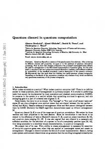
Threshold. There are two types of threshold within the cluster, the topological one in V and thresholds from |Ai and |Y i-state distillation in S. An estimate pVc to the topological threshold is found in numerical simulation of finite-size lattices, pVc = 7.5 × 10−3 . The result of the simulation is displayed in Fig. 10.

11

(21)

Figure 10: Numerical simulation for the topological threshold in V . The curves are best fits taking into account finite size effects of the lattice size l. Beyond the smallest lattices, these finite size effects quickly vanish, and the curves intersect in a single point to a very good degree of accuracy. The value of p at the intersection gives the threshold.

The recursion relations for state distillation, in the limit of negligible topological error, are to A 3 Y Y 3 lowest contributing order ǫA l+1 = 35(ǫl ) (c.f. [30]) and ǫl+1 = 7(ǫl ) . The corresponding distillation thresholds expressed in terms of the physical error rate p are 1 1 ≈ 2.8 × 10−2 , pYc = √ ≈ 6.3 × 10−2 . pA c = √ 6 35 6 7

(22)

The topological threshold is much smaller than the distillation threshold, and therefore the former sets the overall threshold for fault-tolerant quantum computation. In our previous paper [5], the non-topological threshold was the smaller one because the ReedMuller quantum code was probed in the error correction mode instead of the error detection mode associated with state distillation [30]. If we include state-distillation into the setting of [5], the fault-tolerance threshold increases to pc = 6.7 × 10−3 ,

(23)

which is the topological threshold2 . The threshold (23) supersedes the result of [5]. Remark 4. The effect of removing the redundant space-like oriented Λ(Z) gates (c.f. Remark 2) 68 Y is to reduce the effective error on the S-qubits. Eq. (20) then is replaced by ǫA 0 = ǫ0 = 15 p. This affects neither the threshold nor the overhead scaling. The distillation threshold increases but it already is the larger one. Also, as will be discussed in the next section, the exponent which governs Y the overhead scaling is a geometric quantity unaffected by the values of ǫA 0 and ǫ0 in Eq. (20).

6

Overhead

We are interested in the operational cost per gate, O3 , as a function of the circuit size Ω. To facilitate the calculation of O3 it is helpful to introduce the notions of the scale factor λ, the defect 2

The value (23) differs from (21) due to minor differences in the error model. Specifically, [5] requires a 2D structure of three or more layers instead of a single one in the present discussion. Consequently, the used operations and the order of operations differ.

12

thickness d, the gate length L, and the gate volume V . In the presented scheme, quantum gates are realized by twisting defects. For that purpose alone, the defects could be line-like structures. Then, the elementary cell of the lattice L constitutes a building block out of which quantum gates and circuits are assembled. However, in such a setting the property of error correction is lost due to the presence of short error cycles. To eliminate such errors the logical elementary cell is rescaled to a cube of λ×λ×λ elementary cells. The cross-section of a defect with the perpendicular plane becomes an area of d × d elementary cells (see Fig. 8b). The gate length L is the total length of defect within a gate, measured in units of the length of the logical cell. We will subsequently use the gate length for an estimate of the gate error remaining after topological error correction. The gate volume V is the number of logical cells that a gate occupies, each consisting of λ3 elementary cells of L. Each elementary cell is built with 16 operations. Let ǫtop (G, λ, d) be the probability of failure for a gate G, as a function of the scale factor λ, defect thickness d and of its circuit layout. The operational overhead O3 (G) is then O3 (G) = 16λ3 VG exp (ǫtop (G, λ, d)Ω) .

(24)

The exponential factor comes from the expected number of repetitions for a circuit composed of Ω gates G. For a given Ω, the overhead should be optimized with respect to choosing λ(Ω) and d(Ω).

6.1

CSS-gates

The simplification for CSS gates is that no S-qubits are involved and all operations are topologically protected. To perform the optimization in Eq. (24) we need to know the gate error ǫtop as a function of G, λ, d. The errors leading to gate failure may either be cycles wrapping around defects of opposite color or relative cycles ending in defects of matching color. The probability of gate failure is exponential in the length of the shortest cycle or relative cycle, and proportional to the number of such error locations. The minimal cycle length is 4(d + 1) and the number of such cycles is equal to the gate length λLG . The minimal length of a relative cycle leading to an error is λ − d. It stretches between two neighboring defect segments one logical cell apart. The number of such relative cycles is at most 2LG λ(d + 1). There are shorter relative error cycles near junctions, but they are homologically equivalent to the identity operation, (25) Thus, the gate failure rate is ǫtop (LG , λ, d) = λLG (exp (−4κ (d + 1)) + 2(d + 1) exp (−κ(λ − d))) .

(26)

We may now use this expression in Eq. (24) and optimize for given computational size Ω. As an example, the operational overhead for the CNOT-gate of Fig. 1 is displayed in Fig. 11. The scaling limit. We now perform the optimization of O3 in (24) with respect to λ, in the limit of large circuit sizes Ω. First, the gate error ǫtop in (26) is minimized when both exponentials in (26) fall off equally fast, i.e. dopt = λopt /5 for large d, λ. Further, the overhead O3 in (24) is minimized near ǫ(λ(Ω)) = 1/Ω. (27) Then λopt ∼ ln Ω/κ, and O3 ∼

ln3 Ω . κ3

13

(28)

1011

Operational overhead (O3)

1010 109 108 107 106 π/8

105

π/4 CNOT

104

1

2

10

4

10

6

10

8

10

10

10

1012

Number of gates (Ω)

Figure 11: Operational overhead as a function of the circuit size. The upper curves are for the gates exp(i π8 Z) and exp(i π4 X), the lower for the CNOT.

6.2

Non-CSS gates

The estimation of the overhead for the non-CSS operation is along the same lines but more complicated, due to the involved magic state distillation. Every level l of distillation is associated with its own scale factor λl and a defect thickness dl . The optimization of O3 thus is over the larger set of parameters Λ = {{λ0 , d0 , λ1 , d1 , ..., λlmax , dlmax }, lmax }. Further, there are now two types of error. First the previously discussed error of topological error correction resulting from non-trivial error-cycles far away from the S-qubits. Second, there is error associated with the S-qubits where topological error correction breaks down. The distillation of states |Ai and |Y i uses S-qubits at the lowest level. |Ai-distillation is based on the [15, 1, 3] Reed-Muller quantum code [30] and the distillation of |Y i on the [7, 1, 3] Steane code. The |Ai-distillation is performed using the circuit displayed in Appendix A, of volume VA and length LA (See Table 1). At each level l it requires 15 states |Ai of level l − 1 and, on average 1705/512 ≈ 3.33 states |Y i. It succeeds with a probability of 1 − 15ǫA l−1 − ǫtop (LA , λl−1 , dl−1 ), where A ǫl−1 is the error of the states |Ai at level l−1. If successful, the residual error in the states |Ai at level A 3 l is ǫA l = 35(ǫl−1 ) + ǫtop (LY , λl−1 , dl−1 ). The distillation for |Y i, of volume VY and length LY , takes 7 states |Y i of the next-lower level, and succeeds with a probability of 1−7ǫYl−1 −ǫtop (LY , λl−1 , dl−1 ). If it succeeds, the residual error is ǫYl = 7(ǫYl−1 )3 + ǫtop (LY , λl−1 , dl−1 ). The above expressions for success probability and residual errors hold to leading order in the A contributing error probabilities ǫA l−1 , ǫl−1 . Further, a gate error cannot simultaneously lead to termination of the circuit and to a residual distillation error. Thus, we overestimate both error probabilities by adding the full weight ǫtop (L, λl−1 , dl−1 ) to them. A and O Y , and the corresponding The operational overheads for state distillation at level l, O3,l 3,l

14

gate CNOT-gate of Fig. 1a (packed) UZ -gate of Fig. 7c UX -gate of Fig. 7d |Y i-distillation circuit |Ai-distillation circuit of Fig. 12

volume V2 = 12 V1,z = 2 V1,x = 4 VY = 120 VA = 336

length L2 = 22 L1,z = 3 L1,x = 4 LY = 120 LA = 362

Table 1: The gate volume and length for various gates and sub-circuits.

Y residual errors ǫA l , ǫl are described by the recursion relation   A 3 V Y A + 1705 , + 16λ O = 1−15ǫA −ǫ 1(L ,λ ,d ) 15 O3,l−1 O3,l A l−1 3,l−1 512 top A l−1 l−1 l−1   1 Y Y = 1−7ǫY −ǫ (L O3,l + 16λ3l−1 VY , 7 O3,l−1 ,λ ,d ) top

l−1

ǫA l ǫYl

=

=

Y

l−1

l−1

(29)

3 35(ǫA l−1 ) + ǫtop (LA , λl−1 , dl−1 ), 7(ǫYl−1 )3 + ǫtop (LY , λl−1 , dl−1 ).

A = O Y = 16, and (20). The initial conditions are O3,0 3,0 The distillation outputs states |Ai and |Y i at level lmax . One such state |Ai and, on average, 1/2 state |Y i is used to implement a gate exp(i π8 Z) via the circuit displayed in Fig. 7a, of volume V1,z and length L1,z . Its overhead is  

1 Y π/8 3 Y A O3 = O3,lmax + O3,lmax + 24(λlmax ) V1,z exp ǫA lmax + ǫlmax + ǫtop (L1,z λlmax , dlmax ) Ω . 2 (30) The operational overhead needs to be optimized over the parameter set Λ. This has been done numerically [32], and the result is shown in Fig. 11. A 3 The scaling limit. First, we compare the two contributions to ǫA l in (29), 35(ǫl−1 ) and ǫtop . 3 If ǫtop is much larger than 35(ǫA l−1 ) it inhibits the convergence of ancilla distillation. Additional distillation rounds are needed which are the most expensive component. If, to the contrary, ǫtop 3 becomes much smaller than 35(ǫA l−1 ) it does not help the ancilla distillation anymore but blows up the size of the logical cell. Therefore, for optimal operational resources, both contributions A are comparable. Then, in the large size limit, ln ǫA l = 3 ln ǫl−1 , λl = 3λl−1 , dl = 3dl−1 . Further, A Y the success probabilities 1 − 15ǫl and 1 − 7ǫl for ancilla distillation quickly approach unity with increasing distillation level l. Therefore, in the large size limit, for the point of optimal operational resources, the recursion relations (29) can be replaced by

       

O3A O3Y λ3 d ln ǫA ln ǫY





       =      

15 0 0

1705 512

7 0



16 VA 16 VY 27 3 3 3

l

      

O3A O3Y λ3 d ln ǫA ln ǫY

       

(31)

l−1

A , O Y ∼ 27l , ln ǫA , ln ǫY ∼ 3l . Then, with ǫ ∼ 1/Ω (27), Thus, O3,l l l 3,l

O3A , O3Y ∼ (ln Ω)3 . 15

(32)

Note that the distillation operations, for the case of perfect CSS-gates, are associated with the more favorable scaling exponents log3 15 ≈ 2.46 and log3 7 ≈ 1.77, respectively. However, in our case the topological error protection of CSS gates must keep step with the rapidly decreasing error of state distillation, by adjusting the scale factor λ. This leads to a scaling exponent of 3 for the CSS operational resources (c.f. Eq. (28)), which dominates the resource scaling of the entire state distillation procedure. Discussion. We have found that there is one dominant exponent which governs the scaling of the operational overhead for all gates from the universal set, O3 ∼ ln3 Ω, c.f. Eqs. (28) and (32). This exponent is a geometrical quantity. Its value, 3, derives from the fact that the cluster state used in the scheme lives in three spatial dimensions, and that errors are identified with line-like objects (1-chains). Details of the implementation such as the volume and length of the distillation circuits play no role for the scaling. This summarizes the main results of this section. Let us now go beyond scaling and look at the pre-factors. Because of the uniform overhead scaling the ratio of operational costs for non-CSS to CSS-gates is constant in the limit of large computational size Ω. Inspection of Fig. 11 shows that this ratio is in disfavor of the non-CSS gates. Without going into much detail, we would like to point out that there is room for improvement Λ(X) here. The ratio O3A /O3 is proportional to VA /d′ 3 . Herein, d′ is the shortest length of an error that goes undetected in the distillation circuit. Its value is constrained by 1 ≤ d′ ≤ d, where d is the distance of the used code (3 for the Reed-Muller quantum code and the Steane code. The code distance d shall not be confused with the defect thickness d introduced earlier in this section.). In the present discussion, c.f. paragraphs preceding Eq. (29), we have used the lower bound d′ = 1 to simplify the error counting. The advise is to replace the Reed-Muller (Steane) quantum code by another [n, k, d] CSS-code for which the encoded gates exp(i π8 Z i ) (exp(i π4 Z i )), i = 1 .. k, are transversal, and with the additional properties of having a large distance d and a good ratio k/n. Such codes need to be searched for systematically. The distillation circuits can be further optimized. The logical circuit depth can be reduced to 3 for |Ai-distillation and 2 for |Y i-distillation, independent of the the code parameters n, k and d. The circuit height 3 remains unchanged. Thus, the circuit volumes per output qubit VA , VY can be reduced to VA = 9(n/k + 1), VY = 6(n/k + 1).

7

Summary and outlook

In this paper we have discussed in detail the error threshold and overhead for universal fault-tolerant quantum computation based on the one-way quantum computer with a three-dimensional cluster state. By conversion of one spatial cluster dimension into time we have reduced the dimensionality of the scheme to two. Also, the described scheme only requires translation-invariant nearest-neighbor Ising interaction among the qubits. These features should facilitate future implementation. We envision cold atoms in optical lattices [7, 8], two-dimensional ion traps [9], quantum dot systems [10] and arrays of superconducting qubits [11] as suitable candidate systems for experimental realization. On a more abstract level, we have initiated the discussion of the topological properties of the defect configurations. We have described a set of transformation rules that allow us to switch between equivalent configurations. We have applied these rules to simplify sub-circuits and to derive circuit identities, by a sequence of operations reminiscent of the Reidemeister moves for link diagrams. There are a host of questions that remain open, from the applied to the abstract. Below a few are listed.

16

• Optimization of the error threshold. With the current implementation of error correction we have exhausted the capabilities of the minimum-weight chain matching algorithm. There is one improvement that promises a noticeable gain. So far, error corrections on the mutually dual lattices L and L run entirely separate. However, errors on L and L are correlated such that error correction could benefit from cross-talk between the two lattices. • Transversality of encoded gates. Motivated in part by the discussion of overhead in Section 6 but a topic of more general theoretical interest is to find further stabilizer codes that posses the capability of performing non-Clifford gates transversally. • Robustness of error threshold. Here we have discussed a logic gate-based error model. What about more physical error models such as, for example, spins coupled to an Ohmic bath? • Connection with the category-theoretic work of Abramsky and Coecke. In this paper we have used an encoding with two holes per logical qubit. There is another encoding that gets by with a single hole, making additional use of the external system boundary. In that other code, for both the primal and the dual defects, the “cups” of Fig. 1b denote the preparation of a Bell state, and the corresponding “caps” Bell measurement. They provide a concrete physical realization of the corresponding abstract elements in the category-theoretic calculus of [33]. Also, the authors of [33] introduce a “line of information flow”. It is represented by the defect strands in our scheme. If the teleportation identity was the only phenomenology supported by the defects we would not get very far in terms of fault-tolerant quantum computation. To this end, it is crucial to have two distinct types of qubits, primal and dual, which interact in a non-trivial manner (7). Now, the question is whether this enlarged phenomenology can be included in the categorytheoretic framework of [33] and whether it enriches that framework. Acknowledgments. RR would like to thank Hans-Peter B¨ uchler, Jiannis Pachos, Almut Beige, Simon Benjamin, Parsa Bonderson, Trey Porto and David Weiss for discussions. KG is supported by DOE Grant No. DE-FG03-92-ER40701. JH is supported by DTO. RR is supported by the Government of Canada through NSERC and by the Province of Ontario through MEDT.

A

Circuit for state distillation

We use a variant of the magic state distillation circuit described in [30], adapted to the QCC . The topological circuit is displayed in Fig. 12. The procedure is this: we start with a Bell state, encode one of its qubits with the Reed-Muller quantum code and measure each of the 15 qubits leaving the encoder in the eigenbasis of Xi − Yi . The Reed-Muller quantum code [30] has the nice property that the X-syndrome can be measured N15 Xi −Yi √ √ = . Therefore, through the local in the X, Y , X + Y and X − Y -basis. Further, X+Y i=1 2 2 X − Y -measurements and classical post-processing we can both learn the X-syndrome and project the encoded qubit of the Bell pair into an eigenstate of X + Y . Thus, we simultaneously project the unencoded qubit into the state X a Z b |Ai, with a, b ∈ {0, 1} depending on the measurement outcomes and on which of the four Bell states was used. We keep this qubit if the above Xsyndrome measurements yield a trivial outcome. In this case, the residual error ǫl is, to leading A 3 order, ǫA l = 35(ǫl−1 ) (c.f. [30]). The local X − Y -measurements are performed by a unitary operation exp(−i π8 Zi ) followed by an Xi -measurement. Each such unitary requires one ancilla |Ai and, with probability 1/2, one additional ancilla |Y i such that one round of magic state distillation performed in this way

17

consumes 15 states |Ai and, on average, 15/2 states |Y i. With a small modification3 , we can reduce the average number of required |Y i-states to 1705/512. The distillation circuit for |Y i-states is constructed in a similar manner. It is based on the Steane code and requires seven input states |Y i in each round.

Figure 12: QCC -realization of the |Ai-state distillation (a). The dots on the defect lines are the ports to connect |Ai- and |Y i states for Z-rotations (c.f. Fig. 7). The main part in the distillation is the encoder for the [15, 1, 3] Reed-Muller quantum code, displayed as a quantum circuit in (b).

Effective error model on L and L

B

After the mapping described in Section 4 the physical setting is in two dimensions. However, the topological error correction is still performed on the three-dimensional lattices L and L. The error model of Section 5, including gate error for one and two-qubit gates, preparation and measurement, effectively results in Z-errors on individual edges and correlated errors on two edges of L or L, respectively. The location of correlated errors is shown in Fig. 13. The effective error channel on time-like edges is


◦2
8 8 p2
[It ] + 15 p2 [Zt ]
◦ 1 − 23 pP [It ] + 32 pP [Zt ] ◦ T1,t = 1 − 15 (33) 1 − 32 pM [It ] + 23 pM [Zt ] . The effective error channel on a space-like edge—horizontal or vertical—is


◦3
◦2 8 8 T1,s = 1 − 15 p2 [Is ] + 15 p2 [Zs ] ◦ 1 − 23 p1 [Is ] + 23 p1 [Zs ] . 3

(34)

N Denote by J the set of subsets of {1, 2, .., 15} such that (including the identity i∈J Xi is an encoded gate N π operation) for all J ∈ J . Then, for the Reed-Muller quantum code, the Clifford unitary i∈J exp(i 4 Zi ) is also π an encoded gate ∀ J ∈ J , namely I or exp(−i 4 Z). Now suppose that after probabilistic implementation of the π/8-phase gates, N π/4-phase gates on a set K ⊂ {1, 2, .., 15} are required. Then, it is equivalent to perform UK⊕J = N π π π ∼ Z ) exp(i i i∈J exp(i 4 Zi ), ∀J ∈ J , modulo local Pauli operators Zi . (Note that exp(i 4 Z)|Ai = X|Ai = |Ai.) i∈K 4 We minimize the support of UK⊕J mod {Zi } by varying J ∈ J . In this way, we reduce the average number of |Y i-states required in a distillation step to 1705/512 ≈ 3.33.

18

Figure 13: The correlated errors (same for on the primal and dual lattice). Shown are horizontal, vertical and time-like faces of L and L. Thick lines indicate error locations. The effective error channel for each of the correlated errors displayed in Fig. 13 is

8 8 p2 [Iab ] + 15 p2 [Za Zb ] . T2 = 1 − 15

(35)

The probability of time-like and space-like individual errors is different. In the error correction procedure this is accounted for by using non-uniform weights in the minimum-weight chain matching algorithm [28]. Likewise, the correlated errors in the boundary of space-like faces are accounted for by including additional diagonal edges.

References [1] E. Knill, R. Laflamme, and W.H. Zurek, Proc. Roy. Soc. London A 454, 365 (1998). [2] D. Aharonov and M. Ben-Or, Proc. 29th Annual ACM Symp. on Theory of Computing, 176 (1997); D. Aharonov and M. Ben-Or, quant-ph/9906129. [3] D. Gottesman, Ph.D. thesis, Caltech (1997), quant-ph/9705052. [4] P. Aliferis, D. Gottesman, and J. Preskill, Quant. Inf. Comp. 6, 97 (2006). [5] R. Raussendorf, J. Harrington, and K. Goyal, Ann. Phys. 321, 2242 (2006). [6] R. Raussendorf and J. Harrington, quant-ph/0610082. [7] O. Mandel et al., Nature 425, 937 (2003). [8] O. Mandel et al., Phys. Rev. Lett. 91, 010407 (2003). [9] W. K. Hensinger et al., Appl. Phys. Lett. 88, 034101 (2006). [10] Y.S. Weinstein, C.S. Hellberg, and J. Levy, Phys. Rev. A 72, 020304(R) (2005). [11] T. Tanamoto et al., Phys. Rev. Lett. 97, 023501 (2006). [12] M. Varnava, D.E. Browne, T. Rudolph, quant-ph/0507036. [13] M.A. Nielsen, quant-ph/0402005; M.A. Nielsen, C. Dawson, quant-ph/0405134. [14] E. Knill, Nature 434, 39 (2005). [15] K. M. Svore, D. P. DiVincenzo, and B. M. Terhal, quant-ph/0604090. [16] A. Kitaev, Ann. Phys. 303 (2003). [17] H. Bombin, M.A. Martin-Delgado, Phys. Rev. Lett. 97, 180501 (2006).

19

[18] H. Bombin, M.A. Martin-Delgado, quant-ph/0610024. [19] J.K. Pachos, quant-ph/0511273 and Int. J. Quant. Inf. (in press). [20] J.K. Pachos, quant-ph/0605068 and Ann. Phys. (in press). [21] R. Raussendorf and H.J. Briegel, Phys. Rev. Lett. 86, 5188 (2001). [22] R. Raussendorf, D.E. Browne, and H.J. Briegel, Phys. Rev. A 68 (2003). [23] S. Bravyi and A. Kitaev, quant-ph/9811052. [24] E. Dennis, A. Kitaev, A. Landahl, J. Preskill, quant-ph/0110143. [25] M. Freedman, Ch. Nayak and K. Walker, cond-mat/0512072. [26] T. Ohno, G. Arakawa, I. Ichinose, T. Matsui, Nucl. Phys. B 697, 462 (2004). [27] K. Takeda, T. Sasamoto and H. Nishimori, J. Phys. A 38, 3751 (2005). [28] J. Edmonds, Can. J. Math 17, 449 (1965). [29] C. Wang, J. Harrington, and J. Preskill, Ann. Phys. 303, 31 (2003). [30] S. Bravyi and A. Kitaev, Phys. Rev. A 71, 022316 (2005). [31] M. Nielsen and I. Chuang, Quantum Information and Computation. Cambridge University Press (2000). [32] R. H. Byrd, P. Lu and J. Nocedal, SIAM Journal on Scientific and Statistical Computing, 16, 5, pp. 1190-1208, (1995). [33] S. Abramsky and B. Coecke, quant-ph/0402130; and Proceedings of the 19th IEEE Conference on Logic in Computer Science (LiCS‘04). IEEE Computer Science Press (2004).

20