Feb 25, 2009 - focus on states that are eigenstates of tenor products of ..... 15: Cluster state stabilizers consistent with the indicated braiding of defects and ...
Topological cluster state quantum computing Austin G. Fowler1 and Kovid Goyal2 1 2
Centre for Quantum Computer Technology, University of Melbourne, Victoria, AUSTRALIA and Institute for Quantum Information, California Institute of Technology, Pasadena, CA 91125, USA (Dated: February 25, 2009)
arXiv:0805.3202v2 [quant-ph] 25 Feb 2009
The quantum computing scheme described in [1, 2], when viewed as a cluster state computation, features a 3-D cluster state, novel adjustable strength error correction capable of correcting general errors through the correction of Z errors only, a threshold error rate approaching 1% and low overhead arbitrarily long-range logical gates. In this work, we review the scheme in detail framing the discussion solely in terms of the required 3-D cluster state and its stabilizers.
I.
INTRODUCTION
Classical computers manipulate bits that can be exclusively 0 or 1. Quantum computers manipulate quantum bits (qubits) that can be placed in arbitrary superpositions α|0i √ + β|1i and entangled with one another (|00i + |11i)/ 2 [3]. This additional flexibility provides both additional computing power and additional challenges when attempting to correct the now quantum errors in the computer. An extremely efficient scheme for quantum error correction and fault-tolerant quantum computation is required to correct these errors without making unphysical demands on the underlying hardware and without introducing excessive time overhead and thus wasting a significant amount of the potential performance increase. This paper is a simplified review of the quantum computing scheme of [1, 2]. This scheme has a number of highly desirable properties. Firstly, it possesses a threshold error rate of 0.75%, meaning arbitrarily large computations can be performed arbitrarily accurately provided the error rates of qubit initialization, measurement, oneand two-qubit unitary gates are all less than 0.75%. This is particularly remarkable since only nearest-neighbor interactions between qubits are required. Furthermore, arbitrarily distant pairs of logical qubits can be interacted with time overhead growing only logarithmically with separation. This property enables quantum algorithms to be implemented very efficiently [4]. We have previously reviewed this scheme in 2-D [5], framing the discussion solely in terms of manipulating the stabilizers [6] of the surface code [7]. Here we review the scheme as a pure cluster state computation [8] in 3-D, again focusing on stabilizers, without making reference to the surface code or using the somewhat inaccessible language of topology and homology. To further ensure broad accessibility, no prior familiarity with cluster state quantum computation or stabilizers is assumed. There are many reasons to seriously consider a 3-D cluster state approach to quantum computing. Such an approach is quite natural for optical [9, 10] and possibly optical lattice [11, 12] based quantum computing. In both cases, for practical reasons, the 3-D cluster state would be generated and consumed slice by slice as the computation proceeds, with just a small number of slices,
possibly just one or two, unmeasured at any given time. A particularly appropriate technology for generating and measuring such a 3-D cluster state is the photonic module [13]. A detailed architecture making use of the photonic module to explicitly implement 3-D topological cluster state quantum computing has been proposed [14]. An independent ion trap architecture tailored to topological cluster states has also been proposed [15]. The existence of such architectures underscores the need for an accessible introduction to the underlying computation model. The discussion is organized as follows. In Section II, we briefly described stabilizers and cluster states. In Section III, we describe the topological cluster state and give a brief overview of what topological cluster state quantum computing involves. Section IV describes logical qubits in more detail and how to initialize them to |0L i and |+L i and measure them in the ZL and XL bases. State injection, the non-fault-tolerant construction of arbitrary logical states, is covered in Section V. Logical gates, namely the logical identity gate and the logical CNOT gate, are carefully discussed in Section VI along with their byproduct operators. Section VII describes the error correction procedure. Section VIII concludes and discusses some open problems.
II.
STABILIZERS AND CLUSTER STATES
A stabilizer [6] can be thought of as a convenient notation for representing a state. Instead of writing |0i, we can write Z — shorthand for √ the +1 eigenstate of Z. Instead of |ψi = (|00i+ |11i)/ 2, we can write ZZ, XX — the simultaneous eigenstate of these operators. We will focus on states that are eigenstates of tenor products of I, X, Y , Z. Not all states can be described as simultaneous eigenstates of lists of such tensor products, but a sufficiently wide range for our purposes can be. The result of applying a unitary gate U to a state |ψi is U |ψi. If |ψi is an eigenstate of M , the new state U |ψi can be written as U M U † U |ψi, implying U |ψi is an eigenstate of U M U † . Given a list of stabilizers, we can thus track the effect of gates simply by manipulating this list. Of particular interest will be the controlled-Z gate CZ which satisfies CZ† = CZ , CZ (I ⊗ X)CZ = Z ⊗ X, CZ (I ⊗ Z)CZ = I⊗Z, CZ (X⊗I)CZ = X⊗Z and CZ (Z⊗I)CZ =
2 Z ⊗ I. The action of CZ on any other stabilizer can be determined by multiplying these relations. A cluster state [16], or more generally a graph state [17], can be defined constructively as any state obtained by starting with a collection of qubits in |+i then applying CZ gates to one or more pairs of qubits. For example, given three qubits in |+i, or equivalently the three stabilizers XII, IXI, IIX, we can form a 1-D cluster state by applying two CZ gates to obtain the stabilizers XZI, ZXZ, IZX. Note that CZ gates commute. In general, a cluster state is characterized by stabilizers of the form Xi ⊗qj ∈nghb(qi) Zj , where Xi acts on qubit qi , Zj acts on qubit qj and nghb(qi ) denotes the set of qubits connected to qi by CZ gates.
III.
a.)
b.)
TOPOLOGICAL CLUSTER STATES
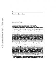
A topological cluster state is a 3-D cluster state with a specific underlying structure. Fig. 1a shows a single cell of a topological cluster state. This cell is tiled in 3-D. Fig. 1b shows a simplified picture of an 8-cell topological cluster state. The wireframe cubes as well as the central shaded region have exactly the same form as Fig. 1a. A topological cluster state can thus be thought of as of two interlocking cubic lattices. We arbitrarily label one of these lattices the “primal” lattice and the other the “dual” lattice. The boundaries of the lattice are also labeled primal or dual according to whether they consist of primal or dual cell faces. If we call the eight wireframe cells of Fig. 1b primal cells, then the lattice has only primal boundaries. If we consider the product of the six stabilizers centered on the six face qubits of Fig. 1a, we find that all Z operators cancel, leaving us with a cell stabilizer that is the tensor product of X on each face qubit. This implies that if we measure each of the face qubits in the X basis, with 0 corresponding to measurement of the +1 eigenstates of X and 1 the -1 eigenstate, we will obtain six bits of information with even parity since the individual X measurements commute with the cell stabilizer and hence the state remains a +1 eigenstate of the cell stabilizer. A string of bits with odd parity tells us that one or more errors have occurred locally. This is how errors are detected. Error correction will be discussed in Section VII. For the moment we simply claim that erroneous measurement results can be corrected arbitrarily well given a sufficiently large topological cluster state and sufficiently low physical error rates. Errors are also defined to be primal or dual according to whether they occur on primal or dual face qubits. Logical qubits are associated with pairs of “defects” — regions of qubits measured in the Z basis. A defect must have a boundary of a single type. There are thus two types of defects and logical qubits — primal and dual. Referring to Fig. 2, for both primal and dual logical qubits the initial U-shape or pair of individual beginnings corresponds to initialization, the middle section,
FIG. 1: a.) A 3-D 18 qubit cluster state. Circles denote qubits initialized to |+i, solid lines denote CZ gates. This cell is tiled in 3-D to form the topological cluster state. b.) A cube of eight cells, which we will call primal cells, each of the form shown in part a (qubits suppressed for clarity). Location of a dual cell (shaded) relative to its surrounding primal cells. A dual cell also contains exactly the arrangement of qubits shown part a.
braided with other defects of the opposite type, corresponds to computation and the final U-shape or pair of individual endings corresponds to read-out. Full details will be given in later sections. Logical operators XL and ZL correspond to a ring or chain of single-qubit Z operators encircling a single defect or connecting the pair of defects. Examples of such rings and chains are shown in Fig. 2. An important point that will become clearer in Section IV is that these rings and chains must be periodically chosen throughout the computation — they cannot be defined in a consistent manner as arbitrary rings and chains since different rings and chains are not equivalent. Furthermore, the logical operators cannot be defined at all during braiding. We shall always choose primal ZL to be a chain connecting two primal defects and dual ZL to be a ring encircling a single dual defect. The definitions of primal and dual XL can be inferred from Fig. 2. Computation makes use of “correlation surfaces” — large cluster state stabilizers connecting logical operators. For example, two rings of Z operators encircling the same defect can be connected with a tube of X operators such that a cluster state stabilizer is formed as shown in Fig. 3. Similarly, two chains of Z operators connecting
3 XL
primal
XL
XL
ZL
ZL
a.)
ZL
X Z
ZL
dual
ZL XL
ZL
Z
X
ZL
XL
XL
XL
MZ XL
primal
XL ZL
ZL
time
b.) X Z
FIG. 2: The definitions of primal and dual ZL and XL — all rings or chains of Z operators. Note that the logical operators are undefined during braiding.
Z
MZ
two defects can be connected with a surface of X operators bordered by Z operators as shown in Figs. 4–5. More complicated defect geometries lead to more complicated correlation surfaces. Fig. 6 shows two logical qubits braided in such a way that ZL on the lower logical qubit connects to ZL ZL on both logical qubits — one of the four mappings associated with logical CNOT. Section VI gives full details of the logical identity and logical CNOT gates.
IV.
LOGICAL INITIALIZATION AND MEASUREMENT
We now move on to the details of topological cluster state quantum computing, focusing on the initialization and measurement of logical qubits in this section. We wish to be able to initialize logical qubits to |0L i and |+L i, the +1 eigenstates of ZL and XL . Take note that deforming a logical operator does not, in general, give an equivalent logical operator. For example, Fig. 7 shows two different chain operators. If the lattice is in the +1 eigenstate of the first chain, it will be in the (−1)MX eigenstate of the second chain, where MX is the result of the indicated X basis measurement. This issue can only be avoided by periodically choosing, by hand, specific rings and chains to represent primal and dual ZL and XL . The correlation surfaces connecting these logical operators can, however, take any shape consistent with the defects in the lattice. To permit concrete discussion, we shall choose one dimension of the topological cluster state to be “simulated time” and arrange the defects of logical qubits not currently being braided to be parallel and in the direction of simulated time as shown in Fig. 8. Note that we define a single time step to correspond to the measurement of a single layer of the cluster state. We define a primal qubit
FIG. 3: Correlation surfaces beginning and ending with rings of Z operators. a.) Red qubits are associated with Z operators, blue qubits with X operators. The collection of red and blue qubits and their associated operators is a cluster state stabilizer. Green highlighting indicates qubits measured in the Z basis, forming a defect. b.) Schematic representation. The surface of X operators can be arbitrarily deformed whereas we keep the initial and final rings of Z operators fixed.
to be in the |+L i state if in a single even time step it is in the simultaneous +1 eigenstate of each of the two operators consisting of a ring of single qubit Z operators encircling and on the boundary of each defect. Similarly, the simultaneous −1 eigenstate of these two boundary operators is defined to be |−L i. There is some redundancy in the way we have defined |+L i and |−L i. It would have been sufficient to focus on a single ring of Z operators around a single defect. Indeed, applying both of these Z rings simultaneously is the logical identity operation — XL is just one of these rings, although it does not matter which ring. For later convenience, when we do not wish to specify which ring, we will use the notation XL . When we need to discuss exactly which operator is being applied, we will write X1 or X2 . Primal qubits can be initialized to |+L i up to byproduct operators via a measurement pattern similar to that shown in Fig. 9. Measuring the indicated qubits in the X basis leaves the defects in either the +1 or −1 eigenstate of X1 and X2 depending on the parity of the associated X measurements. If we denote the parity (sum mod 2) of the X measurements associated with X1 by s1 , the state of the logical qubit after initialization will be Z1s1 Z2s2 |+L i, with ZL = Z1 Z2 and
4
X Z
Z
X
MZ
MZ
FIG. 4: A correlation surface beginning and ending with chains of Z operators. Red qubits are associated with Z operators, blue qubits with X operators. The collection of red and blue qubits and their associated operators is a cluster state stabilizer. Green highlighting indicates qubits measured in the Z basis, forming defects.
dual MZ
X
ZL
Z
Z MZ
primal
FIG. 5: Schematic representation of Fig. 4. The surface of X operators can be arbitrarily deformed provided the Z operators inside the defect remain in the defect. The initial and final chains of Z operators are kept fixed.
{X1 , Z1 } = {X2 , Z2 } = 0. The operators Z1 and Z2 , while not physical unless at least one additional primal boundary is present in the system, are useful for keeping track of byproduct operators affecting a single defect. If an additional primal boundary is present, these operators can be represented by chains of Z starting on each defect and ending on this additional boundary. Note that in the absence of errors all surfaces of X measurements bounded by either X1 or X2 will have the same parity, as the X stabilizer associated with the six faces of a single cell can be used to arbitrarily deform a surface without changing its parity. This implies that the initialization procedure is well-defined and fault-tolerant when used in conjunction with the error correction described in Section VII. Primal qubits can also be initialized to |0L i up to byproduct operators via a measurement pattern similar to that shown in Fig. 10. We choose ZL to be any specific chain of Z in an odd time slice connecting two sections of defect. The parity s of the X and Z measurements in time slices earlier than the chosen logical operator determines the byproduct operator XLs .
ZL
ZL
time FIG. 6: A more complicated arrangement of defects and a correlation surface consistent with the arrangement. The connection of ZL with ZL ZL is suggestive of a CNOT gate, described in detail in Section VI.
a.) Z
b.) Z
MX
FIG. 7: Two nonequivalent chain operators. The second chain operator will have an eigenvalue (−1)MX times the eigenvalue of the first chain operator.
5
Z Z
Z
Z
Z
Z Z
Z
Z ZL
Z
X1 X2 1
0
2
4
3
5
6
time
FIG. 8: A primal qubit consisting of two primal defects with XL = X1 = X2 and ZL indicated.
b.)
X1
a.) X
Z
ΨL = Z1s1Z2s2 +L
primal error chain
Z
X
X2
X
X X
Z
Z
X
X1
Z
Z1
Z
X
X2
s1
X
X X
Z2 s2
Z
Z
FIG. 9: Initializing a primal qubit to the |+L i state. After the indicated X measurements, the two defects are left in known eigenstates of their associated XL operators, X1 and X2 , which are both rings of single-qubit Z operators.
As drawn, Fig. 10 is not fault-tolerant. The defect is too narrow to provide any information about errors on the internal qubits measured in the Z basis. Fig. 11 shows a larger defect and examples of odd parity five sided dual cells resulting from errors on qubits inside the defect. For operations to be fault-tolerant, defects must have minimum cross-section 2 × 2 cells. In addition to demonstrating that primal qubit initialization to |0L i can be made fault-tolerant, Fig. 11 shows how appropriate error information is extracted on the surface of a primal defect to permit dual error correction to continue and vice versa. Furthermore, note that Z measurements deeper inside the defect than the outermost layer are not used in any part of the computation or error correction procedure and as such their results
can be discarded. Dual qubit initialization, expressed in terms of dual cells, looks absolutely identical to primal qubit initialization. The only difference lies in the interpretation of what the initialization procedures mean. A dual measurement pattern of the form shown in Fig. 9 initializes the dual qubit to |0L i. Similarly, a dual measurement pattern of the form shown in Fig. 10 initializes the dual qubit to |+L i. The definitions of all X and Z logical and byproduct operators are also reversed. With logical qubits and logical operators defined, we can now discuss logical errors. In Fig. 9, any chain of primal errors, which can be thought of as Z errors on the underlying qubits before measurement or X basis measurement errors, that connects the two defects is unde-
6
a.)
b.)
dual error ring
ΨL = XsL 0L X1
ZL Z Z Z
Z
X Z
s
Z
X Z
X
X2
ZL
Z
FIG. 10: Initializing a primal qubit to the |0L i state. After the indicated Z and X measurements, the U-shaped defect is left in a known eigenstate of the ZL operator, which is a specific chosen chain of single-qubit Z operators.
FIG. 11: Three examples of X or MZ errors on qubits measured in the Z basis inside a defect. The leftmost examples are errors on the first layer of qubits inside the defect which can be both detected and corrected by determining the parity of five sided dual cells touching the error. The rightmost example is sufficiently deep inside the defect that no nontrivial stabilizers intersect it and therefore the error can be ignored.
tectable and changes the state of the logical qubit from |+L i to |−L i. To make this unlikely, defects must be kept well separated. In Fig. 10, any ring of dual Z and MX errors encircling one of the defects is undetectable and changes the state of the logical qubit from |0L i to |1L i. To make this unlikely, defects must have a sufficiently large perimeter. The situation is similar for dual qubits, with the meaning of the two types of logical errors interchanged. Now that we have initialization, logical measurement follows in a straightforward manner. Figs. 9–10, reversed in time can be used to measure the logical operators of a qubit. The parity of the measurement results determines
the sign of the eigenvalue of the logical operator.
V.
STATE INJECTION
We have discussed logical qubit initialization to states |+L i and |0L i, measurement in the XL and ZL bases and logical errors. We now turn our attention to state injection, specifically the preparation of logical states α|0L i + β|1L i. Consider Fig. 12. The first part of the figure shows a single qubit in an arbitrary state. The logical operators XL and ZL correspond to single-qubit X and Z respec-
7 1. XL ZL
+
Ψ X Z
+
+
a.)
Z Z Z
CZ 2.
+
Ψ XL ZL
X Z
Z
X Z
+
X
Z
Z b.) X
CZ 3.
CZ
X
X X
Z X
Z Z
X
Ψ XL ZL
Z
X
X Z
X
Z
FIG. 12: Injecting an arbitrary state into a four-qubit cluster state. Information about the original state can be obtained from the parity of multiple single-qubit measurements.
X
ZX X X
c.)
X X X
tively. The second part shows the effect of applying a single CZ gate. A two-qubit entangled state is created, however the parity of the two single-qubit measurements XZ gives the same information as the single-qubit measurement X before the CZ gate — XZ is our new XL operator. The CZ gate transforms +1 eigenstates of X into +1 eigenstates of XZ. The third part of the figure includes a further two qubits. The essential idea is that cluster state stabilizers centered on the second, third and fourth qubits can be used to extend the logical operators so they involve more qubits. Consider Fig. 13. The enlarged qubit is the initial location of the arbitrary state. The three parts of the figure show ZL and XL = X1 = X2 after state injection. The parity of the results of measuring the indicated qubits in the indicated bases gives the same information as singlequbit measurements on the initial state. Note that the forms of ZL , X1 , X2 differ from those shown in Fig. 8, where they were simple rings and chains instead of the sheets and socks shown in Fig. 13. This is acceptable as all qubits associated with single-qubit operators in black are measured in the same basis during computation implying application of these single-qubit operators would have no effect. Nevertheless, the full form of the logical operators is important as only from the full form can it be seen that the logical operators anticommute. Furthermore, measuring the single-qubit operators in black introduces logical byproduct operators. Let λZ , λ1 , λ2 denote the parities of the measurements indicated in black in the three parts of Fig. 13. After measurement we will be left with the state XLλZ Z1λ1 Z2λ2 |ψL i. Note that since state injection always begins with a single unprotected qubit, any state injection procedure, including Fig. 13, is inherently non-fault-tolerant. If the enlarged qubit is prepared in an arbitrary state
X
Z
Z
X
X
X X X
Z
Z
FIG. 13: Full form of a.) ZL , b.) X1 , c.) X2 after state injection.
α|0i + β|1i before being entangled with its neighboring qubits, an arbitrary logical state α|0L i + β|1L i can be obtained. In practice, it is likely that the cluster state will be prepared first, implying that the enlarged qubit can only be rotated in the Z basis as such rotations commute with the controlled-Z operators used to construct the cluster state. Rotation before measurement could be replaced with measurement in a rotated basis. Either way, this √ would limit the class of injectable states to (|0i + eiθ |1i)/ 2. VI.
LOGICAL GATES
Only two logical gates, the identity gate and the CNOT gate, are required to complete the universal set of gates. These logical gates can be understood by examining their action on logical operators. For example, an ideal logical identity gate will have the property XL 7→ XL , ZL 7→ ZL . Consider Fig. 14. The upper row shows X1 , X2 followed by these same operators multiplied by a tubular cluster state stabilizer. Measuring the indicated qubits in the X basis results in new logical operators X1′ = (−1)s1 X1 , X2′ = (−1)s2 X2 . Similarly, the lower row relates input and output ZL via ZL′ = (−1)sZ ZL . These logical operator mappings correspond to a logical
8 identity gate with byproduct operators that maps logical ′ states according to |ψL i = (IL )Z1s1 Z2s2 XLsZ |ψL i. Logical CNOT operates in a similar manner. An ideal CNOT maps control and target operators according to Xc 7→ Xc Xt , Xt 7→ Xt , Zc 7→ Zc , Zt 7→ Zc Zt . Consider Fig. 15. The dual qubit is the control and the primal qubit is the target. From the figure it can be seen that Xd 7→ (−1)λXd Xd X1p , X1p 7→ (−1)λX1p X1p , X2p 7→ (−1)λX2p X2p , Z1d 7→ (−1)λZ1d Z1d , Z2d 7→ (−1)λZ2p Z2d , Zp 7→ (−1)λZp Z2d Zp . This corresponds to logical CNOT with byproduct operators mapping logical states according to λ
λ
λZ1d λZ2d λZp ′ |ψL i = CX ZdλXd Z1pX1p Z2pX2p X1d X2d Xp |ψL i. (1)
We do not yet quite have what we need — a logical CNOT between two primal qubits. Consider Fig. 16a [2]. This shows how an additional primal and dual ancilla qubit can be used to simulate logical CNOT between two primal qubits. Essentially, the first CNOT and associated measurement converts the control primal qubit into a dual qubit, the second CNOT performs the necessary logical operation and the third CNOT converts the dual qubit back into a primal qubit. Fig. 16b shows a braiding of defects equivalent to Fig. 16a and a simplified braiding is shown in Fig. 16c [2].
VII.
TOPOLOGICAL CLUSTER STATE ERROR CORRECTION
Topological cluster state error correction is conceptually simple. As discussed in Section III, measuring the six face qubits of a given cell in the X basis should yield six bits of information with even parity. Odd parity cells indicate the presence of errors. If we have a pair of cells with odd parity, we can connect the cells with a path running from face qubit to face qubit, then bit-flip the measurement results associated with the path. This will ensure every cell in the lattice has even parity once more. If we have many cells with odd parity, we can use an efficient classical algorithm, namely the minimum weight matching algorithm [18], to pair up the cells using paths with minimum total length. Applying bit-flips to the measurement results along these paths again results in every cell having even parity. There are, however, many important issues left unanswered by the above paragraph. Errors can occur in chains. A lattice with 64 cells and a number of errors is shown in Fig. 17. Only cells at the endpoints of error chains have odd parity (indicated by thick lines). No information about the path of the error chain is provided. The boundaries of the lattice also require special consideration. Fig. 17 shows a primal lattice of primal cells with primal boundaries containing primal errors. If an endpoint of a chain of at least two primal errors is located on a primal boundary, the boundary cell containing this endpoint will still have even parity. Primal error chains
that begin and end on primal boundaries are thus undetectable and have the potential to cause logical errors as discussed in Section IV. Fig. 18 contains examples of primal error chains connected to primal boundaries. Fig. 18 also contains dual boundaries — lattice boundaries that pass through the centers of primal cells. A primal error chain connected to a dual boundary is always detectable as it changes the parity of the boundary cell containing the endpoint. Dual cells are used in an identical manner to primal cells, meaning they also detect the presence of Z or MX errors on their face qubits. Fig. 19 shows a dual error chain starting and ending on dual boundaries. In an analogous manner to primal error chains, the parity of the dual boundary cells containing the chain endpoints remains unchanged. Primal and dual error correction occur independent of one another. It may seem strange that both appear to only focus on Z and MX errors. An X error that occurs just before an MX measurement has no effect on the measurement result or the underlying cluster state after the measurement. An X error that occurs during the preparation of the cluster state, as shown in Fig. 20, is equivalent to one or more Z errors on the neighboring qubits as well as an X error just before measurement. As before, we can ignore the X error, and the error correction scheme deals with Z errors. We are now in a position to describe how correction proceeds. Note that only the classical measurement results will be corrected, not any remaining unmeasured qubits. Without loss of generality, let us focus on primal errors. The procedure for correcting dual errors is analogous. Suppose we have a connected lattice of (primal) cells with both primal and dual boundaries. Identify one dimension of the lattice as simulated time. Suppose we measure all qubits in the lattice up to some given simulated time t in the X basis and classically determine which cells in the measured region have odd parity. We need an algorithm to match odd parity cells with each other and with primal boundaries such that there is a high probability the matching corresponds to the errors that caused the odd parity cells. We have already mentioned that the algorithm we will use is called the minimum weight matching algorithm [18]. The minimum weight matching algorithm takes a weighted graph with an even number of vertices and produces a spanning list of disjoint edges with the property that no other list has lower total weight. The cells with odd parity become half the vertices we will feed into the algorithm. For every vertex in this list we add a vertex corresponding to the nearest point on the nearest primal boundary. We make an almost complete graph of these vertices according to the following rules: all boundary vertices are connected to all other boundary vertices with edge weight zero, odd parity cell vertices are connected to all odd parity cell vertices with edge weight equal to the sum of the absolute value of the differences of their three coordinates measured in cells, and odd parity cell
9 X1 MX X1
s1
s2
X1=(-1) X1
X2
X2=(-1) X2
MX
X2 Z1
Z2
MX
s
ZL=(-1) ZZL
ZL
X1
X2
ZL
MZ
FIG. 14: The logical identity gate. Red lines and dots indicate Z operators, blue lines indicate X operators. Measuring all qubits in the middle panels in the indicated bases results in a mapping between logical operators with byproduct operators dependent on the parity of the measurement results.
λXd dual
Xd
Xd
λX1p X1p
primal
X1p
X1p
X2p
X2p
λX2p
λZ1d dual
Z1d
Z1d
Z2d
Z2d
Z2d
λZ2d λZp primal
Zp
Zp
FIG. 15: Cluster state stabilizers consistent with the indicated braiding of defects and connecting the indicated logical operators in a manner corresponding to logical CNOT with byproduct operators.
vertices are connected to their nearest boundary vertex with edge weight equal to the number of cells that need to be passed through to reach the boundary plus one. When this graph is processed by the minimum weight matching algorithm, the resulting edge list is highly likely to enable correction of the odd parity cells in a manner that does not introduce logical errors. The classical measurement results along an arbitrary path connecting the relevant pairs of cells are bit-flipped resulting in all measured cells having even parity. Note that in a large computation such corrective bit-flips would only be applied
between pairs of vertices such that at least one vertex of the pair is located at a time earlier than some t − tc where tc depends on the size of the computation. This is to ensure that odd parity cells close to t have a chance to be matched with appropriate partner cell, which may not yet have been measured.
10
a.)
ancilla 0L
control out
control in
MZ
dual ancilla +L
MX
target in
target out
ancilla 0L
control out
control in
MZ
dual ancilla +L
MX
b.)
c.)
target in
target out
control in
control out
target in
target out
FIG. 16: a.) Circuit comprised of logical gates described in the text that simulates logical CNOT between two primal qubits. b.) Equivalent braiding of defects. c.) Equivalent simplified braiding of defects.
FIG. 17: A cluster state comprised of 64 primal cells of the form shown in Fig. 1a. Three different Z or MX error chains of length 1, 2 and 3 are indicated by thick lines and enlarged qubits. Cells with odd parity are indicated with thick bounding lines. Most of the qubits in the cluster state have not been drawn for clarity.
VIII.
CONCLUSION
We have presented a thorough review of [1, 2], discussing how a specific 3-D cluster state can be used to perform general error correction despite only detecting Z and MX errors directly and detailing fault-tolerant ini-
FIG. 18: A cluster state with both primal boundaries and dual boundaries, which consist of primal cells cut in half. Examples of the observable parity effects of primal error chains connected to the two types of boundaries are included with odd parity cells indicated by thick bounding lines.
FIG. 19: An undetectable dual error chain connecting two dual boundaries.
tialization of |0L i and |+L i, ZL and XL measurement, √ non-fault-tolerant preparation of (|0L i+eiθ |1L i)/ 2, and fault-tolerant implementations of the logical identity gate and logical CNOT. By making use of state distillation [5, 19, 20], this set of gates is sufficient to enable universal fault-tolerant quantum computation. Further work is required to determine the level of qubit loss the scheme can tolerate and the dependence of the threshold error rate on qubit loss.
11
X +
IX.
ACKNOWLEDGEMENTS
X MX
+ + +
Z
+
Z
FIG. 20: Quantum circuit showing how X errors occurring at any point during the preparation of the cluster state are equivalent to potentially multiple Z errors and an X error just before measurement in the X basis, which can be ignored.
[1] R. Raussendorf and J. Harrington, Phys. Rev. Lett. 98, 190504 (2007), quant-ph/0610082. [2] R. Raussendorf, J. Harrington, and K. Goyal, New J. Phys. 9, 199 (2007), quant-ph/0703143. [3] M. A. Nielson and I. L. Chuang, Quantum Computation and Quantum Information (Cambridge University Press, Cambridge, 2000). [4] R. V. Meter and K. M. Itoh, Phys. Rev. A 71, 052320 (2005), quant-ph/0408006. [5] A. G. Fowler, A. M. Stephens, and P. Groszkowski, arXiv:0803.0272 (2008). [6] D. Gottesman, Ph.D. thesis, Caltech (1997), quantph/9705052. [7] S. B. Bravyi and A. Y. Kitaev, quant-ph/9811052 (1998). [8] R. Raussendorf, D. E. Browne, and H. J. Briegel, Phys. Rev. A 68, 022312 (2003), quant-ph/0301052. [9] E. Knill, R. Laflamme, and G. J. Milburn, Nature 409, 46 (2001), quant-ph/0006088. [10] W. J. Munro, K. Nemoto, and T. P. Spiller, New J. Phys. 7, 137 (2005), quant-ph/0507084. [11] G. K. Brennen, C. M. Caves, P. S. Jessen, and I. H. Deutsch, Phys. Rev. Lett. 82, 1060 (1999), quant-
We are much indebted to Robert Raussendorf for extensive and illuminating discussions. KG is supported by DOE Grant No. DE-FG03-92-ER40701.
ph/9806021. [12] P. Jaksch, H.-J. Briegel, J. I. Cirac, C. W. Gardiner, and P. Zoller, Phys. Rev. Lett. 82, 1975 (1999), quantph/9810087. [13] S. J. Devitt, A. D. Greentree, R. Ionicioiu, J. L. O’Brien, W. J. Munro, and L. C. L. Hollenberg, Phys. Rev. A 76, 052312 (2007), arXiv:0706.2226. [14] S. J. Devitt, A. G. Fowler, A. M. Stephens, A. D. Greentree, L. C. L. Hollenberg, W. J. Munro, and K. Nemoto, arXiv:0808.1782 (2008). [15] R. Stock and D. F. V. James, arXiv:0808.1591 (2008). [16] H. J. Briegel and R. Raussendorf, Phys. Rev. Lett. 86, 910 (2001), quant-ph/0004051. [17] W. D¨ ur, H. Aschauer, and H.-J. Briegel, Phys. Rev. Lett. 91, 107903 (2003), quant-ph/0303087. [18] W. Cook and A. Rohe, INFORMS J. Comput. 11, 138 (1999). [19] S. Bravyi and A. Kitaev, Phys. Rev. A 71, 022316 (2005), quant-ph/0403025. [20] B. W. Reichardt, Quant. Info. Proc. 4, 251 (2005), quantph/0411036.