Topology Design in Time-Evolving Delay-Tolerant Networks with Unreliable Links Minsu Huang∗ ∗
Siyuan Chen∗
Fan Li†
Yu Wang∗
Department of Computer Science, University of North Carolina at Charlotte, Charlotte, NC 28223, USA. † School of Computer Science, Beijing Institute of Technology, Beijing, 100081, China.
Abstract—With possible participation of a large number of wireless devices in delay tolerant networks (DTNs), how to maintain efficient and dynamic topology becomes crucial. In this paper, we study the topology design problem in a predictable DTN where the time-evolving network topology is known a priori or can be predicted. We model such network as a weighted space-time graph with both spacial and temporal information. Links inside the space-time graph are unreliable due to either the dynamic nature of wireless communications or the rough prediction of underlying human/device mobility. The aim of our topology design problem is to build a sparse space-time structure such that (1) for any pair of devices, there is a space-time path connecting them with the reliability larger than a required threshold; (2) the total cost of the structure is minimized. We first show that this problem is NP-hard, and then propose several heuristics which can significantly reduce the total cost of the topology while maintain the “reliable” connectivity over time.
I. I NTRODUCTION In delay tolerant networks (DTNs), the lack of continuous connectivity, network partitioning, long delays, unreliable time-varying links, and dynamic topology pose new challenges in design of DTN protocols. Recently, several DTN routing schemes [1]–[3] have been proposed to take the intermittent connectivity and time-varying topology into consideration. In addition, different mobility study [4], [5] and graph modeling [6], [7] have been conducted for DTNs to understand the underlying social and temporal characteristics of the network participants. However, there is little research on how to maintain a cost-efficient and reliable topology of DTNs. Network topology is always a critical issue in design of any networking systems. For different network applications, network topology can be designed or controlled under different objectives (such as power efficiency, fault tolerance, and throughput maximization). Topology control protocols have been well studied in wireless networks [8]. The focus of previous research is mainly on how to construct a cost-efficient structure from a static and connected topology. However, in DTNs, the underlying topology is lack of continuous connectivity which makes existing topology control algorithms useless. Therefore, how to efficiently maintain a dynamic The work of M. Huang, S. Chen, and Y. Wang is supported in part by the US National Science Foundation (NSF) under Grant No. CNS-0915331 and CNS-1050398. The work of F. Li is partially supported by the National Natural Science Foundation of China under Grant 60903151, Beijing Natural Science Foundation under Grant 4122070 and Scientific Research Foundation for the Returned Overseas Chinese Scholars, State Education Ministry. Y. Wang (
[email protected]) is the corresponding author.
topology in DTNs becomes crucial, especially with the participation of a large number of wireless devices. In this paper, we study the topology design problem in a time-evolving and predictable DTN. DTNs often evolve over time: changes of network topology can occur if nodes move around. For certain type of DTNs, the temporal characteristics of topology could be known a priori or can be predicted from historical data. For example, it is easy to discovery the temporal pattern of topology for a DTN formed by either public buses [9] or satellites [10] which have fixed tours and schedules, or a mobile social network [5] consisting of students who share fixed class schedules. A recent study [11] on human mobility also shows that a 93% potential predictability can be achieved in human mobility predication. For this kind of time-evolving and predictable DTNs, the space-time graph model [12], instead of the static graph model, can be used to capture both the space and time dimensions of the dynamic network topology and to enable the emulation of any “storeand-forward” DTN routing methods. Given such a spacetime graph including all possible temporal and spacial links, the topology design problem aims to find a subgraph which maintains the connectivity over time between any two devices while minimizing the cost. In our recent study [13], [14], we have proposed several heuristics for the basic topology design problem in timeevolving and predictable DTNs . Those methods all assume that the predication of future links are perfect and links are reliable for communications, i.e., the packet delivery over these spacial or temporal links is guaranteed and without errors. This is clearly too optimistic since in practice, the wireless communications are unreliable due to the lossy nature of wireless channels. In addition, even though certain type of network mobility could be predicated based on user behavior or historical data, the link predication could be inaccurate sometime. Therefore, in this paper, we remove the strong assumptions on reliable links and perfect predication. Instead, for each spacial or temporal link in the space-time graph, we assume it has a probability to reflect its “reliability”, either based on link quality estimation or mobility predication. Larger the reliable probability of a link, higher chance the DTN transmissions over that link to be successful. Therefore, given the weighted space-time graph, the new reliable topology design problem (RTDP) aims to find a subgraph in which the reliability of DTN routing between any two devices is guaranteed larger than a required threshold and the total cost
of topology is minimized. In this paper, we show that this new topology design problem is NP-hard and propose five heuristics which can significantly reduce the total cost of network topology while maintaining the DTN reliability over time. For our best knowledge, this paper is the first attempt to study topology design for time-evolving networks with unreliable links. space v1
v4
v1 v4
v3 v5
v4
v2
v2
v3
v2
v2
v5
v3 v1
v3
v4
v1
v5
v5 t=1
t=2
t=3
(a)
t=4
time
v10
v11
v14
v20
v21
v24
v30
v31
v34
v40
v41
v44
v05
v15
v45
t=1
t=2
t=3 t=4
(b)
Fig. 1. A time-evolving DTN and its corresponding space-time graph: (a) the time-evolving topology of a DTN (a sequence of snapshots); (b) the corresponding space-time graph G, where a space-time DTN path from the source v2 to the destination v5 is highlighted in blue.
II. M ODELS , A SSUMPTIONS , AND T HE P ROBLEM A. Modeling Time-evolving Networks: Space-time Graphs Assume that V = {v1 , · · · , vn } be the set of all individual nodes (wireless devices) in the network over a period of time T . Here, time is divided into discrete and equal time slots, e.g. {1, · · · , T }. Since positions of individual nodes and the topology co-evolve over time, a sequence of static graphs can be defined over V to model the interactions among nodes in the time-evolving DTN during certain time slot. Fig. 1(a) illustrates such an example. Let Gt = (V t , E t ) be a directed graph representing the snapshot of the network at time slot t −−→ and a link vit vjt ∈ E t represents that node vi can communicate to vj at time t. Then, the dynamic network is described by the union of all snapshots {Gt |t = 1 · · · T }. However, such sequence of static graphs is not directly useable in the analysis of DTN routing protocols. Some of the snapshots may not be connected graphs at all (e.g., the first three snapshots in Fig. 1(a)), which makes routing task over them challenging. In some existing DTN protocols, an aggregated graph over {Gt } is used, where an edge between a pair of nodes represents these two nodes have interacted at certain point during the time period T . The weight of such an edge could be the fraction of the occurrence over the historical period of that interaction, i.e., a contact probability. Several DTN routing protocols [1], [3] estimate this contact probability based on past contact history and use it to select relay nodes. However, such aggregated view discards temporal information about the timing and order of interactions, which may cause failure of delivery or bad performances. In this paper, we adopt the space-time graph [12] to model the time-evolving DTNs. We convert the sequence of static graphs {Gt } into a space-time graph G = (V, E), which is a directed graph defined in both
spacial and temporal spaces. Fig. 1(b) illustrates the spacetime graph of the same network in Fig. 1(a). In the spacetime graph G, T + 1 layers of nodes are defined and each layer has n nodes, thus the whole vertex set V = {vjt |j = 1, · · · , n and t = 0, · · · , T } and there are n(T + 1) nodes in G. Two kinds of links (spatial links and temporal links) are −−−−→ added between consecutive layers in E. A temporal link vjt−1 vjt (those horizontal links in Fig. 1(b)) connects the same node vj across consecutive (t − 1)th and tth layers, which represents the node carrying the message in the tth time slot. A spatial −−−−→ link vjt−1 vkt represents forwarding a message from one node → t vj to its neighbor vk in the tth time slot (i.e., − v− j vk ∈ E ). By defining the space-time graph G, any communication operation in the time-evolving network can be simulated on this directed graph. As the blue path shown in Fig. 1(b), a space-time DTN path from v20 to v54 shows a particular DTN routing strategy to deliver the packet from v2 to v5 in the network: v2 holds the packet for 1st time slot, then passes it to v3 at t = 2, etc. We can define the connectivity of a space-time graph which is different from that of a static graph. Definition 1: A space-time graph H is connected over time period T if and only if there exists at least one directed path for each pair of nodes (vi0 , vjT ) (i and j in [1, n]). This guarantees that any packet can be delivered between any two nodes in the network over the period of T . Note that a connected space-time graph does not require the connectivity in every snapshot. Hereafter, we assume that the original space-time graph G is connected over time period T . For each direct link e ∈ E, we further assume that there is a cost c(e), representing the cost associated with transiting a message over that link (transiting from one node to the other node over a spacial link or holding the message within one node over a temporal link). The total cost of a space-time graph c(H) is defined as the summation of costs of all links in H, i.e., X c(H) = c(e). (1) e∈H
PcH (u, v)
is defined as the path from u to The least cost path v in H with thePminimum total cost. Its total cost is denoted by cH (u, v) = e∈P H (u,v) c(e). c
B. Reliability of DTN Topology over Unreliable Links To consider the reliability of lossy wireless links or unperfected link predications, we also define a reliable probability r(e) for each link e ∈ E, which represents the probability of a successful data transmission over link e. The unreliability of the link could come from either link failure due to lossy wireless signal or poor predication of future links. Here, we assume that the reliable probability of each link can be obtained through link estimation techniques at the link and physical layers [15] or mobility predication techniques [16]. Fig. 2(a) illustrates a simple space-time graph with just two devices. The label of each link e is the pair of cost and reliability, i.e., (c(e), r(e)). For example, in the first time slot, −−→ the cost of spacial link va0 vb1 is 3 and its reliability is 0.6. Given
va0 (2,0.5) va1 (2,0.5)
va2
va0 (2,0.5) va1 (2,0.5)
va2
va0 (2,0.5) va1 (2,0.5)
va2
(3,0.6)
(3,0.6)
(3,0.6)
(3,0.6)
(3,0.6)
(3,0.6)
(1,0.8)
(1,0.8)
(1,0.8)
(1,0.8)
(1,0.8)
(1,0.8)
vb0 (5,1.0) vb1 (5,1.0)
vb2
(a) G
vb0 (5,1.0) vb1 (5,1.0)
(b) H1
vb2
vb0 (5,1.0) vb1 (5,1.0)
vb2
(c) H2
Fig. 2. Examples of reliable topology design: (a) the original space-time graph G with cost 22 and reliability 0.36; (b) H1 with cost 6 and reliability 0.25; and (c) H2 with cost 12 and reliability 0.36. Here, links are labeled by (cost, reliability), and green links are removed links from G.
the reliability of each link, we can then define the reliability of a path P or a structure H. In this paper, we only consider the reliability for single-copy DTN routing where only one copy of each message is propagated in the network. Thus, the resulting propagation path of a message is basically a single space-time path in G. Given a path P (u, v) connecting nodes u and v, the reliability of P (u, v) is the production of reliability of all links in that path. For example, the path va0 → va1 → vb2 in Fig. 2(a) has reliability of 0.5 × 0.8 = 0.4. For a given routing topology H, we can define the most reliable path PrH (u, v) as the path from u to v in H with the highest reliability. Let rH (u, v) = Πe∈PrH (u,v) r(e) be the reliability of path PrH (u, v). For example, between va0 and vb2 in Fig. 2(a), va0 → vb1 → vb2 is the most reliable path with reliability of 0.6 × 1.0 = 0.6. Then the reliability of the topology H is defined as follows r(H) = min rH (vi0 , vjT ). 1≤i,j≤n
(2)
The reliability of structures shown in Fig. 2(a), (b) and (c) are 0.36, 0.25 and 0.36 respectively. Notice that it is easy to calculate r(H) given H by using any shortest path algorithms.
Hardness of RTDP: The topology design problem for space-time graph even without reliability requirement is much harder than the one for a static graph. For a static graph without time domain, a minimum spanning tree can achieve the goal of keeping connectivity with minimal cost. However, simply applying the spanning tree in each snapshot or over the entire space-time graph is not a direct solution. First, the graph in each snapshot may not be connected at all. On the other hand, a spanning tree or forest of the whole space-time graph connects each node in every snapshot, which is not necessary and a waste of many links. Plus the reliability requirement, the RTDP becomes more challenging. In [13], we have proved that the topology design problem without reliability requirement is NP-hard. Since such topology design problem is a special case of RTDP when γ = 1, RTDP is also NP-hard. The RTDP is different with the standard space-time routing [12], [17], which only aims to find the most cost-efficient space-time path for a pair of source and destination. The topology design problem aims to maintain both cost-efficient and connected space-time routing topology for supporting reliable DTN transmissions between all pairs of nodes. III. H EURISTICS OF R ELIABLE T OPOLOGY D ESIGN
C. Reliable Topology Design Problem We now can define the reliable topology design problem (RTDP) on weighted space-time graphs as follows. Definition 2: Given a connected space-time graph G, the aim of reliable topology design problem (RTDP) is to construct a sparse space-time graph H, which is a subgraph of the original space-time graph G, such that (1) H is still connected over the time period T ; (2) the reliability is larger than or equal to a predefined threshold γ; and (3) the total cost of H is minimized. Notice that generally speaking denser space-time topology leads to better connectivity and reliability but more expensive in term of total cost. Therefore, the topology design aims to find a topology with certain reliability guarantee while minimizing the cost. If the threshold γ is a constant, the reliability requirement itself covers the basic connectivity, since it is obviously a much stronger requirement than basic connectivity. Once again, we assume that the original spacetime graph G is connected and has reliability larger than γ. Fig. 2(b) and (c) show two sub-topologies of Fig. 2(a) with different costs and reliability. Note that these topologies are still connected over time, i.e., every node can find a space-time path to any other node.
Since RTDP over space-time graphs is NP-hard, we now propose five different heuristics to construct a sparse structure that fulfills the connectivity and reliability requirements over time. The first three heuristics are based on minimum cost reliable routing, while the other two are based on greedy algorithms. For all algorithms, the inputs are the original graph G and reliability requirement γ ≤ 1, and the output is a subgraph H of G. A. Heuristics Based on Min Cost Reliable Path One natural idea to construct a low-cost reliable subgraph, which guarantees the route reliability between any two nodes over the time period T , is keeping all the minimum cost reliable paths from vi0 to vjT for i, j = 1, · · · , n in G. Here the minimum cost reliable path connecting u and v, denoted G by Pcr (u, v), is the path with the least cost among all paths between u and v which have reliability larger than or equal to γ. Obviously, if we can find such paths for every pair of source and destination, the union of all of them satisfies the reliability requirement of our topology design problem. However, to find the shortest path with additional constrains in a graph itself is also a well known NP-hard problem, called restricted shortest path problem [18]. Therefore, in this paper, we use one of
the existing heuristics for restricted shortest path, BackwardForward method (BFM) by Reeves and Salama [19]. The basic idea of Backward-Forward method is quite simple. Assume we want to find a reliable path from s to t. BFM first determines the least-cost path (LCP) and the most reliable path (MRP) from every node u to t. It then starts from s and explores the graph by concatenating two segments: (1) the sofar explored path from s to an intermediate node u, and (2) the LCP or the MRP from node u to t. BFM simply uses Dijkstras algorithm with the following modification in the relaxation procedure: a link uv is relaxed if it reduces the total cost from s to v while its approximated end-to-end reliability obeys the reliability constraint. The computational complexity of the BFM is basically three times that of Dijkstra’s algorithm. G Let PBF M (u, v) be the resulting path from u to v based on G BFM. Notice that PBF M (u, v) is not optimal for restricted shortest path. However, based on simulation study by Kuipers et al. [20], BFM is one of the most efficient methods among all existing methods, it has small execution time and often generates good quality path compared with the optimal. Algorithm 1 Union of Min Cost Reliable Path (UMCRP) 1: H ← φ; X = {(vi0 , vjT )} for all integer 1 ≤ i, j ≤ n. 2: for all pairs (vi0 , vjT ) ∈ X do G 0 T 3: Find the “minimum” cost reliable path PBF M (vi , vj ) in G using Backward-Forward method. G 0 T 4: if e ∈ PBF / H then M (vi , vj ) and e ∈ 5: H = H ∪ {e}. 6: return H
Algorithm 2 Greedy with Min Cost Reliable Path (GMCRP) 1: H ← φ; X = {(vi0 , vjT )} for all i and j in [1, n]. 2: while X 6= φ do 3: Find the minimum cost reliable paths for every pair nodes in X using BFM in G, and assume PBF M (vi0 , vjT ) has the least cost among these paths. 4: if e ∈ PBF M (vi0 , vjT ) then 5: H ← e; c(e) ← 0. 6: X ← X − (vi0 , vjT ). 7: return H
With Backward-Foward method, our first heuristic approach is to find a “minimum” cost reliable path for each pair of source and destination and take the union of them to form the subgraph which guarantee the overall reliability. Algorithm 1 shows the detailed algorithm. Its time complexity is O(n2 T (log(nT ) + n)) since we only need to compute n2 minimum cost reliable paths of G (with O(nT ) nodes and at most O(n2 T ) links). This can be easily achieved by running 3n times of Dijkstra’s algorithm whose complexity is O(nT (log(nT ) + n)). Hereafter, we refer this method as union of minimum cost reliable path algorithm (UMCRP). However, the structure built by the above method may contain more links than necessary. Therefore, we propose a new greedy algorithm (as shown in Algorithm 2) to further improve the performance. The basic idea is as follows. We aim to connect n2 pair of nodes in X. In each round we pick the minimum cost reliable path between a pair nodes in X which is the minimum among all minimum cost reliable paths connecting any pair of nodes in X. Then we add all links in this path into H, clear the costs of these links to zeros, and remove this pair from X. This procedure is repeated until all pair nodes (vi0 , vjT ) are guaranteed to be connected by reliable paths in H. It is obvious that the output of this method is much sparser than the one of UMCRP method. We refer this method as greedy method based on minimum cost reliable path (GMCRP). The time complexity is O(T n5 + T n4 log(T n)) since 3n times of Dijkstra’s algorithm are running on the space-time graph in each round for n2 rounds. The third method basically combines the least cost path and the minimum cost reliable path. It includes two steps. In the first step, we connect n2 pair of nodes in X = {(vi0 , vjT )} for all integer 1 ≤ i, j ≤ n by adding all of the least cost paths between them. After this step, we have a structure H which connects all pairs of (vi0 , vjT ) but may not satisfy the reliability requirements yet. In the second step, for each pair (vi0 , vjT ), we calculate its reliability in H. If the cost of rH (vi0 , vjT ) is less than γ, we directly add the links in the minimum cost reliable path between this two nodes in G into H. See Algorithm 3 for detail. Hereafter, we denote this method as LCP/MCRP. Both steps of LCP/MCRP need n2 ·O(n2 T (log(nT )+n)) time since they both run computation of shortest paths for O(n2 ) rounds. Therefore, the total time complexity is O(n4 T (log(nT ) + n)). B. Greedy-based Heuristics
Algorithm 3 Least Cost Path or Min Cost Reliable Path (LCP/MCRP) 1: H ← φ; X = {(vi0 , vjT )} for all integer 1 ≤ i, j ≤ n. 2: for all pairs (vi0 , vjT ) ∈ X do 3: Find the least cost path PcG (vi0 , vjT ) in G. 4: if e ∈ PcG (vi0 , vjT ) and e ∈ / H then 5: H = H ∪ {e}. 6: for all pairs (vi0 , vjT ) ∈ X do 7: if rH (vi0 , vjT ) < γ then G 0 T 8: Add all links e ∈ PBF / H. M (vi , vj ) into H if e ∈ 9: return H
Both the fourth and fifth algorithms are based on the same greedy principle, deleting or adding edges in order and checking whether the reliability is achieved or void. The basic idea of the fourth method is deleting edges from input graph (either the original graph G or the output graph from the first two algorithms) in a decreasing order based on link cost. Link vit vjt+1 is removed if the subgraph H without this link can still achieve reliability of γ. Algorithm 4 shows the detailed algorithm, and we denote it as GDL hereafter. The time complexity analysis is straightforward. The sorting could be done in O(n2 T log(n2 T )) with O(n2 T ) links. The for-loop includes n2 T rounds of computations of shortest paths. Thus,
Algorithm 4 Greedy Algorithm to Delete Links (GDL) 1: H ← G. 2: Sort all links in link set E of G based on their costs. 3: for all e ∈ E (processed in decreasing order of costs) do 4: if r(H − {e}) ≥ γ then 5: H = H − {e}. 6: return H Algorithm 5 Greedy Algorithm to Add Links (GAL) 1: H ← φ; X = {(vi0 , vjT )} for all integer 1 ≤ i, j ≤ n. 2: for all pairs (vi0 , vjT ) ∈ X do 3: Find the least cost path PcG (vi0 , vjT ) in G. / H then 4: if e ∈ PcG (vi0 , vjT ) and e ∈ 5: H = H ∪ {e}. 6: for all e ∈ G − H (in increasing order of costs) do 7: if r(H) < γ then 8: H = H + {e}. 9: return H
the time complexity of this part is O(n4 T 2 (log(nT ) + n)). Therefore, total time complexity of GDL is also in order of O(n4 T 2 (log(nT ) + n)), which is much higher than those of methods based on minimum cost reliable path. Note that since the outputs of our first two algorithms are much sparser than the original graph but can guarantee the reliability, if we use them as the input of GDL it can save certain computation cost. The fifth algorithm is also a greedy algorithm but processes links in the reverse order compared with the fourth algorithm. It starts with building a connected sparse structure and then adds more links to satisfy the reliability requirement. It also includes two steps. In the first step, again we take the union of all least cost paths between (vi0 , vjT ) for all integer 1 ≤ i, j ≤ n as H. In the second step, remaining links are processed in the increasing order of cost. Link vit vjt+1 is added to H if the current subgraph H cannot achieve reliability of γ yet. See Algorithm 5 for detail. Hereafter, we denote this method as GAL. The complexity of GAL is the same as the one of GDL (O(n4 T 2 (log(nT ) + n))) since the second step is almost the same with GDL and the first step cost less time. IV. S IMULATIONS To evaluate our proposed algorithms devoted to the RTDP problem we have conducted extensive simulations over randomly generated networks. We implement and test the following six algorithms: UMCRP (Alg 1), GMCRP (Alg. 2), LCP/MCRP (Alg. 3), GDL (Alg. 4), GAL (Alg. 5), and ULCP. Here, ULCP is the union of least cost paths from vi0 to vjT for i, j = 1, · · · , n), which maintains the connectivity over time but cannot guarantee the reliability. We use ULCP as a reference. In all simulations, we take three metrics as the performance measurement for any algorithm devoted to RTDP: •
Total Cost: the total cost of the constructed P topology H (output of the algorithm), i.e., c(H) = e∈H c(e).
Total Number of Edges: the total number of edges in H, i.e., |H|. Here, |G| denotes total edge number of G. H 0 T • Reliability: r(H) = min1≤i,j≤n r (vi , vj ). The objective of topology design is to construct topologies with small total cost, small edge number and larger reliability. The underlying time-evolving networks are randomly generated from random graph model. We first generate a sequence of static random graphs {Gt } with 10 nodes, spreading over 10 time slots. For each time slot t, the static graph Gt is generated using the classical random graph generator. For each → pair of nodes vi and vj , we insert edge − v− i vj with a fixed t probability δ into G . Small value of δ leads to a sparse DTN, and δ = 1.0 implies that the topology in each time slot is a complete graph. After generating the sequence of {Gt }, we convert it into the corresponding space-time graph G. The cost and reliability of each inserted edge are randomly chosen from 1 to 50 and from 0.8 to 1, respectively. For each setting, we generate 100 random time-evolving networks and report the average performance of our algorithms among them. For the first set of simulations, we increase the network density by rising δ from 0.2 to 0.8, and keep reliability requirement γ at 0.6. Fig. 3(a) and 3(b) show the ratios between the total cost/number-edges of the generated graph H and that of the original graph G with increasing δ. This ratio implies how much saving achieved by the topology design algorithm, compared with the original network. From the results, all algorithms can significantly reduce the cost of maintaining the connectivity. Even with the least density (δ = 0.2), all algorithms except for GAL can save more than 70% cost and around 65% edges. When the network is denser, the saving of topology design is larger. For δ = 0.8, more than 85% cost is saved. Comparing all methods, we can find the following observations. (1) ULCP has the least cost since it only guarantee the connectivity while other proposed algorithms guarantee the reliability; (2) GAL has the largest cost due to simply adding many low-cost links; (3) GMCRP achieves smaller cost than UMCRP since it reuse some links in previous rounds; (4) LCP/MCRP’s cost is between ULCP’s and UMCRP’s since it combines both LCP and MCRP; (5) Overall, GDL and GMCRP have the best costs among the proposed five methods. Fig. 3(c) shows the reliability of each structure generated by all methods. Clearly, LCP is the only algorithm that cannot satisfy the reliability requirement γ = 0.6. It is an algorithm only for maintaining the connectivity over time. All other five algorithms can always achieve the desired reliability, and they have very close performance in term of reliability. But considering their costs, GDL, GMCRP, LCP/MCRP are better choices. When G is sparse (e.g. δ = 0.2), its reliability is just over 0.6. In that case, our proposed algorithms remove around 70% edges but still keep the reliability at the desired level. This clearly demonstrates the power of topology design. In the second set of simulations, we fixed the network density δ = 0.5 and run our algorithms with different reliability requirement γ increasing from 0.3 to 0.6. From results shown in Fig. 4, we can observe that tighter reliability requirement results in higher cost and larger number of •
1
1
1
0.9
0.9
0.9
0.6
ratio of edge number
ratio of total cost
0.7
0.5
0.4
0.3
0.7
0.6
0.4
0.3
0.2
0.1
0.1
0.3
0.4
0.5
0.6
0.7
0 0.2
0.8
0.8
0.5
0.2
0 0.2
UMCRP GMCRP LCP/MCRP GDL GAL ULCP
0.8
unicasting reliability
UMCRP GMCRP LCP/MCRP GDL GAL ULCP
0.8
0.7
0.6
0.5
UMCRP GMCRP LCP/MCRP GDL GAL ULCP G
0.4
0.3
0.2
0.1
0.3
0.4
δ
0.5
0.6
0.7
0 0.2
0.8
0.3
0.4
δ
0.6
0.7
0.8
δ
(b) |H|/|G|
(a) c(H)/c(G)
0.5
(c) r(H)
Fig. 3. Simulation results on random networks with different density and γ = 0.6. (a)-(b): The cost (or edge number) of H is divided by the cost (or edge number) of G, which shows how much saving achieved by proposed methods. (c): The reliability r(H) shows the reliability of H. 1
0.7
0.6
0.5
0.4
0.3
0.7
0.6
0.8
0.5
0.4
0.3
0.7
0.6
0.5
0.4
0.3
0.2
0.2
0.2
0.1
0.1
0.1
0 0.3
0.35
0.4
0.45
0.5
0.55
0.6
0 0.3
0.35
0.4
γ
Fig. 4.
0.45
γ
(a) c(H)/c(G)
UMCRP GMCRP LCP/MCRP GDL GAL ULCP G
0.9
UMCRP GMCRP LCP/MCRP GDL GAL ULCP
0.8
ratio of edge number
ratio of total cost
0.8
1
0.9
UMCRP GMCRP LCP/MCRP GDL GAL ULCP
unicasting reliability
1
0.9
(b) |H|/|G|
0.5
0.55
0.6
0 0.3
0.35
0.4
0.45
0.5
0.55
0.6
γ
(c) r(H)
Simulation results on random networks with fixed network density δ = 0.5 and varying reliability requirement γ.
edge-usage of our topology algorithms. When the reliability requirement becomes looser, the restriction on removing links becomes weaker. In the extreme case with γ = 0, our RTDP converges to the basic topology design problem [13] which only preserves the connectivity. Notice that performances of LCP do not affect by the reliability requirement. In addition, GAL performs better when the reliability requirement is small. V. C ONCLUSION We study reliable topology design problem in a predictable time-evolving DTN with unreliable links modeled by a probabilistic space-time graph. We propose a set of new heuristics which can not only maintain the connectivity and reliability of paths over time but also significantly reduce the cost of topology. Simulation results from random networks demonstrate the efficiency of our methods. We believe that this paper presents the first step in exploiting topology design for time-evolving DTNs with unreliable links. R EFERENCES [1] Q. Yuan, I. Cardei, and J. Wu, “Predict and relay: an efficient routing in disruption-tolerant networks,” in ACM MobiHoc ’09, 2009. [2] T. Spyropoulos, et al., “Spray and wait: an efficient routing scheme for intermittently connected mobile networks,” in ACM WDTN ’05, 2005. [3] A. Lindgren, A. Doria, O. Schel´en, “Probabilistic routing in intermittently connected networks,” Mob. Comp. Comm. Rev., 7(3):19–20, 2003. [4] J. Leguay, T. Friedman, and V. Conan, “Evaluating mobility pattern space routing for DTNs,” in IEEE INFOCOM, 2006.
[5] V. Srinivasan, et al., “Analysis and implications of student contact patterns derived from campus schedules,” in ACM Mobicom, 2006. [6] E.M. Daly and M. Haahr, “Social network analysis for routing in disconnected delay-tolerant manets,” in ACM MobiHoc, 2007. [7] T. Hossmann, et al., “Know thy neighbor: towards optimal mapping of contacts to social graphs for DTN routing,” in IEEE INFOCOM, 2009. [8] Y. Wang, “Topology control for wireless sensor networks,” book chapter, Sensor Networks & Applications (eds. Y. Li et al.), Springer, 2007. [9] X. Zhang, J. Kurose, B.N. Levine, D. Towsley, and H. Zhang, “Study of a bus-based disruption-tolerant network: mobility modeling and impact on routing,” in ACM MobiCom ’07, 2007. [10] S. Burleigh and A. Hooke, “Delay-tolerant networking: an approach to interplanetary internet,” IEEE Commun. Mag., 41(6):128–136, 2003. [11] C. Song, Z. Qu, N. Blumm, and A.-L. Barabasi, “Limits of predictability in human mobility,” Science, 327:1018–1021, 2010. [12] S. Merugu, M. Ammar, and E. Zegura, “Routing in space and time in networks with predictable mobility,” GIT, Tech. Rep., CC-04-07, 2004. [13] M. Huang, S. Chen, Y. Zhu, et al., “Topology control for time-evolving and predictable delay-tolerant networks,” in IEEE MASS, 2011. [14] M. Huang, S. Chen, et al., “Cost-efficient topology design problem in time-evolving delay-tolerant networks,” in IEEE Globecom, 2010. [15] N. Baccour, et al., “A comparative simulation study of link quality estimators in wireless sensor networks,” in IEEE MASCOTS, 2009. [16] W. Su, S. Lee, and M. Gerla, “Mobility prediction in wireless networks,” in IEEE MILCOM, 2000. [17] B.B. Xuan, A. Ferreira, and A. Jarry, “Computing shortest, fastest, and foremost journeys in dynamic networks,” Int’l J. of Foundations of Computer Science, 14(2):267–285, 2003. [18] F. A. Kuipers, “An overview of constraint-based path selection algorithms for QoS routing,” IEEE Communications Magazine, 50–56, 2002. [19] D. S. Reeves and H. F. Salama, “A distributed algorithm for delayconstrained unicast routing,” IEEE/ACM Trans. Netw., 8:239–250, 2000. [20] F. Kuipers, T. Korkmaz, et al., “Performance evaluation of constraintbased path selection algorithms,” IEEE Network, 18:16–23, 2004.