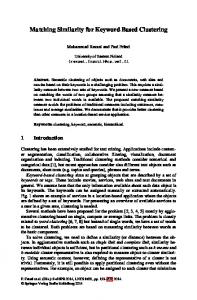
Topology Matching for Fully Automatic Similarity Estimation of 3D Shapes Masaki Hilaga∗ ∗
The University of Tokyo
†
Yoshihisa Shinagawa∗
The Institute of Physical and Chemical Research
Abstract There is a growing need to be able to accurately and efficiently search visual data sets, and in particular, 3D shape data sets. This paper proposes a novel technique, called Topology Matching, in which similarity between polyhedral models is quickly, accurately, and automatically calculated by comparing Multiresolutional Reeb Graphs (MRGs). The MRG thus operates well as a search key for 3D shape data sets. In particular, the MRG represents the skeletal and topological structure of a 3D shape at various levels of resolution. The MRG is constructed using a continuous function on the 3D shape, which may preferably be a function of geodesic distance because this function is invariant to translation and rotation and is also robust against changes in connectivities caused by a mesh simplification or subdivision. The similarity calculation between 3D shapes is processed using a coarse-to-fine strategy while preserving the consistency of the graph structures, which results in establishing a correspondence between the parts of objects. The similarity calculation is fast and efficient because it is not necessary to determine the particular pose of a 3D shape, such as a rotation, in advance. Topology Matching is particularly useful for interactively searching for a 3D object because the results of the search fit human intuition well. Keywords: Computer Vision, Shape Recognition, 3D Search
1
Taku Kohmura†
Introduction and Related Work
Recent developments in modeling and digitizing techniques have made the construction of 3D computer models much easier. This has led to an increasing accumulation of 3D models, both on the Internet and otherwise, and has highlighted the need for development of an efficient technique for searching for a particular 3D object in a data set. This paper proposes a search method called Topology Matching that efficiently, accurately, and automatically estimates a measure of similarity and correspondence between 3D shapes. When dealing with 2D images, techniques have been proposed for recognizing a silhouette or contour curve using properties of shape, such as curvature [10, 15, 19, 24, 27, 34] or using properties of image, such as color, texture or wavelet coefficient [12, 17, 20]. ∗ {garhyla,sinagawa}@is.s.u-tokyo.ac.jp †
[email protected] ‡
[email protected]
Permission to make digital or hard copies of all or part of this work for personal or classroom use is granted without fee provided that copies are not made or distributed for profit or commercial advantage and that copies bear this notice and the full citation on the first page. To copy otherwise, to republish, to post on servers or to redistribute to lists, requires prior specific permission and/or a fee. ACM SIGGRAPH 2001, 12-17 August 2001, Los Angeles, CA, USA © 2001 ACM 1-58113-374-X/01/08...$5.00
‡
Hosei University
Tosiyasu L. Kunii‡ ‡
Kanazawa Institute of Technology
These techniques have been used to conduct searches on 2D multimedia image databases. When dealing with 3D shapes, there are a number of techniques for shape matching and feature extraction, for example, extracting features for a design in feature-based CAD/CAM applications [14, 16, 35, 38], computing a feature from images and matching 3D models in a database for posture estimation or object search in model-based vision [5, 40], and optimizing some measures for registration of 3D shapes [2, 7]. However, these techniques are generally restricted to their specific applications, and inadequate for a general 3D shape search. In order to contruct a 3D shape database, it is first necessary to define a search key on the shapes. Curvature is a possible candidate for this search key, and methods using curvature distribution have provided some good results for uses such as 3D shape pose estimation [11, 18, 22, 35, 39]. However, since curvature is associated with second order derivatives, these techniques are inadequate as a general search key because they are sensitive to noise and small undulations on the object surface, even if a multiresolutional structure is introduced. Other studies have used a global histogram as a search key for a database of 3D shapes [3, 29]. This type of search key is computationally stable and suitable for representing rough features of shapes but cannot, however, estimate local features. In order to handle global and local properties simultaneously, the selected search key must include a concise representation of the shape, must catch the features of the shape well, and must be computed automatically and robustly for a general 3D shape database. In order to satisfy such conditions, we propose using a skeletal structure of a 3D shape as a search key. There have been many studies on the extraction of a skeleton from a 3D shape [8, 9, 32, 41] for use in various applications such as shape deformation, modeling and path planning. One well-known skeletal structure is the medial axis model [4, 8, 9, 32, 34]. However, this model is inappropriate as a search key for 3D shapes because calculating the 3D version of a medial axis has a high computational cost and is sensitive to noise and small undulations. After examining various options, we have chosen a skeleton structure called the Reeb graph as the basis for our search key. The Reeb graph, defined by Reeb [30], is a skeleton determined using a continuous scalar function defined on an object. Reeb graphs have been used for both modeling 3D shapes [33, 36, 26] and visualization [13], and certain particular cases are used in terrain applications [1, 23, 37]. The Reeb graph has a number of characteristics that make it useful as a search key for 3D objects. First, a Reeb graph defined appropriately always consists of a one-dimensional graph structure and does not have any higher dimension components such as the degenerate surface that can occur in a medial axis. Second, by defining the continuous function appropriately, it is possible to construct a Reeb graph that is invariant to translation and rotation, robust against connectivity changes caused by simplification, subdivision and remesh, and resistant against noise and certain changes due to deformation. In particular, we have found that such properties can be provided by using a continuous function based on the distribu-
s3
r2 r0 s0
r 1 s1
s2
r6 r 5 s9 r 4 s6 r 3 s4
s11 s10 s8 s5
s7 n11
n9
n3 n0 n1
n2
n4
Figure 1: Torus and its Reeb graph using a height function tion of geodesic distance. Finally, since a Reeb graph is associated with the value of a continuous function, it is possible to introduce a multiresolutional structure. In Topology Matching, we propose a Multiresolutional Reeb Graph (MRG), which is constructed based on geodesic distance, as a search key. Our use of geodesic distance has been aided by the fact that the computation of geodesic distance between two points has been well studied [6, 21, 25, 28, 31]. The geodesic-based MRG allows a similarity between 3D shapes to be calculated using a coarseto-fine strategy while preserving the topological consistency of the graph structures to provide a fast and efficient estimation of similarity and correspondence between shapes. In section 2, the Reeb graph is described and its extension to a Multiresolutional Reeb Graph (MRG) is proposed. The continuous function used for Topology Matching is defined in section 3. Section 4 explains the implementation and the construction of the MRG. Similarity estimation and its implementation are described in section 5. Section 6 describes the results of an experiment using Topology Matching to search for a 3D object. The paper concludes in section 7 with a discussion of the results and future work.
2
Reeb Graph and Its Multiresolutional Extension
2.1
Reeb Graph
A Reeb graph is a topological and skeletal structure for an object of arbitrary dimensions. In Topology Matching, the Reeb graph is used as a search key that represents the features of a 3D shape. The definition of a Reeb graph is as follows: Definition: Reeb graph Let µ : C → R be a continuous function defined on an object C. The Reeb graph is the quotient space of the graph of µ in C × R by the equivalent relation (X1 , µ(X1 )) ∼ (X2 , µ(X2 )) which holds if and only if • µ(X1 ) = µ(X2 ), and • X1 and X2 are in the same connected component of µ−1 (µ(X1 )). When the function µ is defined on a manifold and critical points are not degenerate, the function µ is referred to as a Morse function, as defined by Morse theory e.g., [33], however, Topology Matching is not subject to this restriction. It is clear that, if the function µ changes, the corresponding Reeb graph also changes. Among the various types of µ and related Reeb graphs, one of the simplest examples is a height function on a 2D manifold. That is, the function µ returns the value of the zcoordinate (height) of the point v on a 2D manifold: µ(v(x, y, z)) = z. Most existing studies have used the height function as the function µ for generating the Reeb graph [33, 1, 23, 36, 37]. Figure 1 shows the distribution of the height function on the surface of a torus and the corresponding Reeb graph. In the left figure,
n6
n10 n7
n8 n5
(a) (b) (c) Figure 2: Multiresolutional Reeb graph using a height function the red and blue coloring represents minimum and maximum values, respectively, and the black lines represent the isovalued contours. The Reeb graph in the right figure corresponds to connectivity information for these isovalued contours.
2.2
Multiresolutional Reeb Graph
This subsection proposes a new Multiresolutional Reeb Graph (MRG). The basic idea of the MRG is to develop a series of Reeb graphs for an object at various levels of detail. To construct a Reeb graph for a certain level, the object is partitioned into regions based on the function µ. A node of the Reeb graph represents a connected component in a particular region, and adjacent nodes are linked by an edge if the corresponding connected components of the object contact each other. The Reeb graph for a finer level is constructed by re-partitioning each region. In Topology Matching, the re-partitioning is done in a binary manner for simplicity. Figure 2 shows an example where a height function is employed as the function µ for convenience of explanation. In Figure 2(a), there is only one region r0 and one connected component s0 . Therefore, the Reeb graph consists of one node n0 which corresponds to s0 . In Figure 2(b), the region r0 is re-partitioned to r1 and r2 , giving connected components s1 and s2 in r1 , and s3 in r2 . The corresponding nodes are n1 , n2 and n3 respectively. According to the connectivities of s1 , s2 and s3 , edges are generated between n1 and n3 , and between n2 and n3 . Finer levels of the Reeb graph are constructed in the same way as shown in Figure 2(c). The MRG has the following properties: Property 1: There are parent-child relationships between nodes of adjacent levels. In Figure 2, the node n0 is the parent of n1 , n2 and n3 , and the node n1 is the parent of n4 and n6 , etc. Property 2: By repeating the re-partitioning, the MRG converges to the original Reeb graph as defined by Reeb. That is, finer levels approximate the original object more exactly. Property 3: A Reeb graph of a certain level implicitly contains all of the information of the coarser levels. Once a Reeb graph is generated at a certain resolution level, a coarser Reeb graph can be constructed by unifying adjacent nodes. Consider the construction of the Reeb graph shown in Figure 2 (b) from that shown in 2 (c) as an example. The nodes {n4 , n6 } are unified to n1 , {n5 , n7 , n8 } to n2 , and {n9 , n10 , n11 } to n3 . Note that the unified nodes satisfy the parent-child relationship. Using these properties, MRGs are easily constructed and a similarity between objects can then be calculated using a coarse-to-fine strategy of different resolution levels as described below.
3
Definition of the Continuous Function µ for Topology Matching
A Reeb graph is always generated by a continuous function µ. If a different function is used as µ, the Reeb graph will change. It is important that the function µ be carefully defined for the application
Figure 5: Resampling and subdivision of a mesh
(a)
where the function g(v, p) returns the geodesic distance between v and p on S. This function µ(v) has no source point and hence stable, and it represents the degree of center or edge on a surface. Since µ(v) is defined as a sum of geodesic distance from v to all points on S, a small value means that a distance from v to arbitrary points on the surface is relatively small, that is, the point v is nearer the center of the object. Here, note that the function µ(v) is not invariant to scaling of the object. To handle this issue, a normalized version of µ(v) is used:
(b)
µn (v) = (c) (d) Figure 3: Examples of the distribution of the function µ and its isovalued contours for Topology Matching: (a) sphere, (b) cube, (c) torus and (d) cylinder.
Figure 4: Example of a deformed shape showing distribution of the function µ in question. For example, in terrain modeling applications or when modeling a 3D shape based on cross sections such as CT images, the height function has been a useful function µ because these applications are strictly bound by height. However, the height function is not appropriate as a search key for identifying a 3D shape because it is not invariant to transformations such as object rotation. Though the use of curvature as the function µ may provide invariance in a rotation, it is also not appropriate for our purposes, because a stable calculation of curvature is difficult on a noisy surface, and small undulations may result in a large change of curvature, causing sensitivity in the structure of the Reeb graph. In order to define a function µ that overcomes such problems, we use geodesic distance, that is, the distance from point to point on a surface. Using geodesic distance provides rotation invariance and resistance against problems caused by noise or small undulations. In one case, Lazarus et al. proposed a level set diagram (LSD) structure [26] in which geodesic distance from a source point is used as the function µ. However, in this case, the function µ is only suitable for constructing a reasonable set of cross sections of a 3D shape. To make a search key for 3D shapes, the source point must be determined automatically and in a stable way, which is a difficult problem. For example, a small change in the shape may result in an entirely different source point, creating an obstacle for the construction of a stable Reeb graph. In order to avoid these difficulties, we construct the function µ at a point v on a surface S as follows:
Z µ(v) =
g(v, p)dS p∈S
(1)
µ(v) − minp∈S µ(p) maxp∈S µ(p)
In this normalization, range(S) = maxp∈S µ(p) − minp∈S µ(p) may also be a candidate for the denominator, however it is not employed because it amplifies errors when range(S) is small, particularly in the case of a sphere, where range(S) = 0. The value minp∈S µ(p) corresponds to a most central part of the object, and a shift can be introduced to initially match the centers of different objects when estimating similarity between them, as described below. Examples of the function µn (v) defined on several primitive objects are shown in Figure 3 where the coloring has the same meaning as Figure 1. Notice that the sphere has a constant value of µn (v) = 0, and more asymmetric shapes have a wider range of values for µn (v). The function µn (v) is particularly useful because it is resistant to the type of deformation shown in Figure 4. This is because the deformation does not drastically change the geodesic distance on the surface. Thus, the normalized integral of geodesic distance is suitable as the continuous function for Topology Matching.
4
Construction of the Multiresolutional Reeb Graph
This section describes how to calculate the function µn (v) and construct the MRG in practice. Here, we focus on constructing the MRG from a triangle mesh (or polyhedron mesh) because meshes are the most common method for representing 3D shapes. Further, a mesh can generally be easily converted to and from other representations such as NURBS surfaces, meta-balls(blobby), subdivision surfaces, etc.
4.1
Calculating the Integral of Geodesic Distance
Methods for calculating an accurate geodesic distance have been well studied [6, 21, 25, 28, 31], however, when calculating the integral of geodesic distance using these methods, the computational cost is quite high. Considering the trade off between computational cost and accuracy, we employ a relatively simple method in which geodesic distance is approximated by Dijkstra’s algorithm based on edge length (described below). However, before using our procedure, the mesh needs to be prepared. In Topology Matching, because a value of the function µn is assigned to each vertex of the mesh, the algorithm will only work well if the distribution of the vertices is fine enough to represent the distribution of the function µn well. It is therefore sometimes necessary to resample the vertices until all edge lengths are less than a threshold p as shown in Figure 5.
u1
v1
1
v3
1
r3
t3
t1 u2
v3
u1
v1
0.75
u3 t2
0.5
u3
u2
0.5
0
(a)
(b) 1
n4 0.75
n4
n2
n3
n2
n1
g(v, bi ) · area(bi )
i
where {bi } = {b0 , b1 , ...} are the base vertices for Dijkstra’s algorithm which are scattered almost P equally on the surface S. area(bi ) is the area that bi occupies, and i area(bi ) equals area(S), the whole area of the surface S. In our procedure, {bi } are selected using the above Dijkstra’s algorithm with two small modifications:
n6
n8
n1
n5
n0 0
n7
0
0
(d) (e) (f) (g) Figure 8: Construction of a Multiresolutional Reeb Graph
Figure 7: Example of bases of geodesic distance and the area of the bases
X
1
0.5
0.25
n0
Equation (1) is then discretely approximated by
1
n3
0.5
0.25
0
(c)
0.75
0.5
Step 5: Repeat Step 3 and 4 until V LIST is empty.
v3
0
1
Step 1: Initialize g(v) = ∞ about all vertices. Step 2: Select a base vertex b, set g(b) = 0, and insert b to V LIST . Step 3: Take the vertex v which has smallest g(v) in V LIST and remove it from V LIST . Step 4: For each vertex va adjacent to v, if g(v) + length(v, va ) < g(va ), update g(va ) = g(v) + length(v, va ) and insert (or reinsert) va to V LIST . Notice that the adjacency of vertices is determined by edges, including short-cut ones.
v2
0.25
Figure 6: Generation of short-cut edges
Dijkstra’s Algorithm for Geodesic Distance:
vx
r0
v2
Further, special edges called “short-cut edges” may need to be added to the mesh. If edges of a mesh are uniform in a certain direction, the accuracy of the calculation of µ(v) is biased, and results in an inaccurate calculation of µn (v). Therefore, short-cut edges are introduced to modify the uniformity by making the directions of edges isotropic. Figure 6 illustrates the algorithm for adding a short-cut edge. First, the triangles t1 , t2 and t3 which are adjacent to the triangle tc are unfolded on the plane of tc . New edges are then generated between each of the vertex pairs but only if an edge is inside the unfolded polygon (< u1 − v1 − u2 − v2 − u3 − v3 >) and has not been previously generated. In Figure 6, the new edges are shown by green and red lines and include (v1 , v2 ), (v2 , v3 ), (v1 , u3 ), (v2 , u1 ) and (v3 , u2 ). In this example, an edge is not added between (v3 , v1 ) since it would be outside the unfolded polygon. The length of a generated edge is the Euclidian distance between the corresponding vertices in the unfolded domain. After the vertex resampling and short-cut edge generation, the geodesic distance of each vertex from a base vertex is calculated using Dijkstra’s algorithm and a binary tree V LIST where the vertices are sorted in ascendant order of g(v).
0.75
r1 0.25
v2
µ(v) =
v1
0.75
r2
tc
va is only inserted (or reinserted) into V LIST at Step 4 if g(va ) is less than a threshold r and, if V LIST is empty at Step 5, an arbitrary unvisited vertex is selected as a new bi , and the procedure is repeated by inserting it into V LIST . Here, area(bi ) is calculated based on the area of faces composed of vertices whose distance from bi is less than r. If the threshold r is smaller, more vertices are selected as {bi }. An increase in the number of base vertices allows a more exact calculation of µ(v) but requires much more computation time. In our implementation, we found that an p r = 0.005 · area(S) generates about 150 base vertices and achieves sufficient accuracy. An example of {bi } and area(bi ) is shown in Figure 7 where the black points on the surface are {bi } and the colored areas correspond to the occupied domains of area(bi ). Finally, the function µn (v) is calculated by normalizing µ(v) as described in section 3 above.
4.2
Construction of the Multiresolutional Reeb Graph
After the calculation of µn (v), the Multiresolutional Reeb Graph (MRG) is constructed. The construction of an MRG is illustrated in Figure 8. In this case, a height function is used as the function µ on a 2D triangle mesh for convenience of explanation. The process is similar when using geodesic distance as the function µ on a 3D shape. We first define the following notation: R-node: A node in an MRG. The red, green and blue circles in Figure 8 are R-nodes, with different colors representing different resolution levels. R-edge: An edge connecting R-nodes in an MRG. The thick black lines in Figure 8 are R-edges. An R-edge can also connect R-nodes of different resolutions. T-set: A connected component of triangles in a region. One T-set corresponds to one R-node (see subsection 2.2). µn -range: A range of the function µn concerning an R-node or a T-set. For example, the µn -range of n2 is [0.5, 0.75) in Figure 8. The construction of the MRG begins with the construction of a Reeb graph having the finest resolution desired. This Reeb graph is constructed by first dividing the domain of the function µn into 1 1 2 K µn -ranges, that is, r0 = [0, K ), r1 = [ K ,K ), ..., rK−1 = K−1 [ K , 1). The fineness of the resolution is determined by the number of µn -ranges K. In Figure 8 (a), the domain is divided into 4 µn -ranges, that is, r0 = [0, 0.25), r1 = [0.25, 0.5), r2 = [0.5, 0.75) and r3 = [0.75, 1).
Second, any triangles lying over the boundaries of the µn -ranges are subdivided so that every triangle belongs to only one µn -range as shown in Figure 8 (b). The position of an inserted vertex is calculated by interpolating the positions of the relevant two vertices in the same proportion as their value of µn (v). For example, as shown in Figure 8 (c), when the triangle composed of v1 , v2 and v3 is divided by the boundary µn (v) = 0.75, a new vertex vx is inserted as follows: vx =
NLIST m2
m0
m4
m2
R:
m5 [0.75, 0.875) m3
m0 m1
m3 [0.5, 0.75) m1 m1 [0, 0.5) n2
v1 (µn (vx ) − µn (v2 )) + v2 (µn (v1 ) − µn (vx )) µn (v1 ) − µn (v2 )
n0
n5
n4
[0.75, 1)
Computational Cost for Constructing the Multiresolutional Reeb Graph
When constructing the MRG, Dijkstra’s algorithm takes O(V log V ) cost where V is the vertex count in the mesh because the size of the binary tree V LIST is O(V ), each insertion to (or removal from) V LIST takes O(log V ) cost, and there are O(V ) iterations. Constructing the T-sets (R-nodes) and connectivities (R-edges) takes O(V ) cost because it is achieved by simply calculating the connected component of the triangles. Therefore, Dijkstra’s algorithm is predominant in the overall computational time. In practice, it occupies approximately 90% of the whole. According to our experiments, using 150 base vertices for Dijkstra’s algorithm gives a sufficient approximation. In this case, an MRG for a mesh of 10,000 vertices can be calculated in approximately 15 seconds with a Pentium II 400MHz processor.
5 5.1
Matching Algorithm Overview
This subsection gives an overview of how similarity is calculated using MRGs. First, for each R-node m, we compute its attribute, called m. ¯ The attribute m ¯ is initially calculated at the finest resolution using the area and the length of the T-set corresponding to the given Rnode as defined below in subsection 5.4, however, more generally, we compute m ¯ =
X
c¯
(2)
c
where c is the child R-node of the R-node m. Thus, the attribute of m is the sum of the attributes of the children of m.
n4
n6 [0.75, 0.875)
n3
n0 n1
4.3
n7 [0.875, 1)
n5
n2
S:
where µn (vx ) = 0.75. Thirdly, the T-sets (connected components of triangles) are calculated in each µn -range, and an R-node is created for each T-set as shown in Figure 8 (d). Fourthly, if two T-sets between adjacent µn -ranges are connected, corresponding R-nodes are connected by an R-edge as shown in Figure 8 (e). This completes the construction of the finest resolution Reeb graph. Next, the Multiresolutional Reeb Graph (MRG) is constructed from the finest resolution Reeb graph by using Property 3 of the MRG as described in subsection 2.2. That is, the MRG is constructed in fine-to-coarse order by unifying adjacent R-nodes while maintaining their parent-child relationships as shown in Figures 8 (e) → (f) → (g), where n5 is the parent of {n0 , n1 }, n6 is the parent of {n2 } etc. While Figure 8 shows only the R-edges connecting R-nodes of the same resolution, there are also R-edges connecting R-nodes of different resolutions that are also calculated at this time. Specifically, the R-edges (n1 , n6 ), (n1 , n7 ), (n2 , n5 ) and (n3 , n5 ) are generated by the connectivities at the boundary µn (v) = 0.5.
m6 [0.875, 1)
m4
n3 [0.5, 0.75) n1 n1 [0, 0.5)
(a)
(b) (c) (d) Figure 9: Overview of the matching algorithm
The similarity between two R-nodes m and n is defined as the similarity between their attributes: sim(m, ¯ n ¯ ). The similarity is defined such that it satisfies the following conditions: 0 ≤ sim(m, ¯ n ¯ ) ≤ sim(m, ¯ m) ¯
(3)
X
(4)
sim(m, ¯ m) ¯ = 1.
m∈R
i.e., sim(m, ¯ n ¯ ) is largest when an R-node is matched with itself and the sum of similarities is 1 if all R-nodes in an MRG R match themselves. Then, the similarity SIM (R, S) between MRGs R and S can be defined as follows: SIM (R, S) =
X
sim(m, ¯ n ¯ ),
m∈R,n∈S
that is, SIM (R, S) is the similarity for a given set of R-node pairs {(m0 , n0 ), (m1 , n1 ), ...}, and it takes a value between [0, 1] with a larger value indicating that the MRGs are more similar. The definition of sim is described in more detail below in section 5.4. Further, because each MRG forms a graph structure, the R-node pairs must also preserve the topological consistency of these graph structures. Therefore, the problem is reduced to finding the R-node pairs that provide the largest value of SIM (R, S) while maintaining topological consistency. To avoid a combinatorial explosion of NP-complexity, in Topology Matching we calculate the similarity using a coarse-to-fine strategy and maintain a list of the R-nodes, N LIST , and a list of matching R-node pairs, M P AIR. Matching Algorithm: Step 1:(Initialization) Insert the coarsest R-nodes of two MRGs R and S to N LIST . Step 2:(Matching) In N LIST , find a matching R-node pair (m ∈ R, n ∈ S) which preserves the topological consistency of the MRG. At the coarsest level, this matching is trivial. The detailed process is described in subsection 5.3. Step 3:(Unpacking) Remove m and n from N LIST and insert (m, n) to M P AIR. Then, if not at the finest resolution, insert the child R-nodes of m and n to N LIST . Step 4:(Loop) If N LIST is not empty, repeat Step 2 and Step 3. Otherwise, calculate SIM (R, S) using sim(m, ¯ n ¯ ) for each element in M P AIR. The calculation of sim(m, ¯ n ¯ ) is described in subsection 5.4.
Figure 9 shows an example of the matching algorithm. In Figure 9 (a), the two R-nodes m0 and n0 are inserted to N LIST (i.e. the
nodes that are not matched yet. Once the R-node is matched, the M LIST is unnecessary because it is not used again. X
R:
m0
5.3
m0 X
m1
m2
m1
m2
matching X
X
S:
n0
n0 X
n1
n2
n1
n2
(a) (b) Figure 10: Propagation of a matching label R-nodes at the coarsest level in the MRG R and S respectively). In Figure 9 (b), (m0 , n0 ) are matched and are thus unpacked to their child R-nodes (m1 , m2 , n1 and n2 ) which are inserted into N LIST . In the next iteration, (m2 , n2 ) are matched and then unpacked as shown in Figure 9 (c), and then in a following iteration (m4 , n5 ) are matched and unpacked as shown in Figure 9 (d). Note that while the N LIST is simply the list of the R-nodes, Figure 9 also shows the associated R-edges for convenience of explanation.
5.2
Topological Consistency of the Multiresolutional Reeb Graph
It is clear that nodes in different ‘branches’ of the Reeb graph should not be matched in order to preserve the topological consistency of the MRGs. The following two rules are introduced to ensure that topological consistency is preserved. The first rule is that the R-nodes can be matched only if they are in the same µn -range and their parents are matched. The latter condition is, however, not applied to the coarsest R-nodes because they do not have a parent. This rule is based on the fact that the µn ranges of two R-nodes are generally the same if they correspond to the same parts of an object. Figure 9 (d) shows an example in which the R-nodes are displayed with their µn -range. m5 can match only with n6 because m5 and n6 have the same µn -range [0.75, 0.875), and their parents m4 and n5 are matched. Notice that m5 would not match any child of n4 because m4 (the parent of m5 ) did not match n4 . The second rule is that R-nodes can only be matched if their M LIST s are the same, where M LIST is a list of the matching labels propagated to that R-node. This rule avoids the matching of nodes in different branches. For example, consider a case of a matching between MRG R and S as shown in Figure 10(a) where the nodes (m0 , n0 ) are matched and we label the matching X. After the matching X, m1 can be matched with either n1 or n2 if the first rule is satisfied although the latter is incorrect. In order to avoid this inconsistency, the matching label X is propagated as shown by the dotted arrows in Figure 10(b), so that m1 , m2 , n1 and n2 are distinguished. That is, m1 can match n1 , but cannot match n2 because X is propagated to m1 and n1 , but is not propagated to n2 . The second rule is implemented by providing each R-node with the matching list, M LIST . In every matching, the matching label is propagated in the direction of a monotonic increase or decrease about the µn -range (i.e., X is not propagated to m2 and n2 in Figure 10(b)), and is appended to the appropriate M LIST s. Thus, R-nodes can only be matched if their M LIST s are the same. Note that the M LIST only needs to be maintained for the R-
Finding the Matching of R-node Pairs
This subsection describes how to find the R-node pairs to be matched, which is the core procedure in the matching algorithm. First, in N LIST , the R-node m whose sim(m, ¯ m) ¯ is the maximum in N LIST is selected as the one side of the matching pair. Thus, the R-node that affects the final result the most is selected. Second, using the two rules of topological consistency, the candidate R-nodes which could match m are selected. That is, a candidate has the same µn -range as m, its parent must match m’s parent, and its M LIST must be equal to that of m. Of course, the candidate must also belong to a different MRG than m. If there is no candidate which can match m, m is removed from N LIST , but nothing is inserted to M P AIR or N LIST , and a matching label is not propagated because m is not matched. The process then returns and repeats the matching steps from the beginning. If there are candidates that can match m, one R-node n is selected from among the candidates using the matching function mat(m, ¯ n ¯ ) (described below) which takes a larger value when there is a better match (m, n). Finally, the matching R-node pair (m, n) (or (n, m)) is returned as the result. Definition of Matching Function mat(m, ¯ n ¯) The matching function mat(m, ¯ n ¯ ) is defined by considering two aspects of similarity. We first introduce the function loss(m, ¯ n ¯) which represents a measure of how the final similarity is decreased by the matching (m, n). loss(m, ¯ n ¯) =
1 {sim(m, ¯ m) ¯ + sim(¯ n, n ¯ )} − sim(m, ¯ n ¯) 2
A larger loss(m, ¯ n ¯ ) means a smaller similarity. We must also define mat(m, ¯ n ¯ ) taking adjacent R-nodes (i.e. the graph structure) into account. Let adj([s, t), m) be the set of R-nodes adjacent to m whose µn -ranges are [s, t). The attribute adj([s, t), m) is then defined as follows:
X
adj([s, t), m) =
a ¯.
a∈adj([s,t),m)
Thus, we may define mat(m, ¯ n ¯ ) as follows: mat(m, ¯ n ¯)
= −loss(m, ¯ n ¯) −
X
loss(adj([s, t), m), adj([s, t), n))
[s,t)
Here, we limit the adj([s, t), m) to the R-nodes in N LIST in order to reduce the computational cost.
5.4
R-node Attribute and Similarity
In Topology Matching, the attribute m ¯ of the R-node m consists of two parameters; i.e., m ¯ = (a(m), l(m)). These parameters a(m) and l(m) are the ratios of the area and the length of the R-node m in the whole object, respectively. While other parameters such as color can also be considered, we introduce a(m) and l(m) as major parameters because they can be easily and stably calculated for any mesh. Their definitions are as follows: a(m): Let area(m) be the area of the T-set corresponding to m, area(S) be the whole area of the object S, and rnum be the
m3
n5
m2
n3
m1
n1
m0
n4 n2 n0
Figure 11: Sensitivity at region boundaries resolution number in the MRG. Then, a(m) is defined as a(m) =
area(m) 1 · , rnum area(S)
1 where rnum is introduced because the relevant part of the object is held by (or incorporated in) rnum R-nodes, each at different resolution levels.
l(m): Let len(m) be the “length” of the R-node m: len(m) = max(m) − min(m) where min(m) and max(m) are the minimum and maximum of µn (v) in m. Note that min(m) and max(m) are not always equal to the µn -range; i.e.,, s ≤ min(m) ≤ max(m) ≤ t when the µn -range is [s, t). The l(m) is defined using len(m): len(m) 1 l(m) = ·P rnum len(n) n where n are the R-nodes of the finest resolution. As described in subsection 5.1, the parameters a(m) and l(m) are first calculated as above at the finest resolution and used to calculate the attributes of the R-nodes at the finest resolution. The attributes for R-nodes at coarser levels are then calculated using equation (2) above. For this purpose, the addition of attributes is defined by m ¯ +n ¯ = (a(m) + a(n), l(m) + l(n)). Notably, l(m) at a coarse resolution can be regarded as a parameter representing the complexity of the graph occupied by m because a larger l(m) means that m is responsible for more R-nodes at the finest resolution. We define the similarity between two attributes as a linear combination of a(m) and l(m). sim(m, ¯ n ¯)
= w · min(a(m), a(n)) +(1 − w) · min(l(m), l(n))
where w (0 ≤ w ≤ 1) controls the weighting of the area and length parameters, and min(x, y) returns the smaller value. Notice that sim(m, ¯ n ¯ ) defined in this way satisfies equations (3) and (4) above.
5.5
Matching at a µn -Region Boundary
One remaining issue is that the structure of an MRG is sensitive to the placement of the region boundaries of the function µn . Figure 11 shows an example in which almost the same objects results in different MRGs due to slight differences in the locations of the region boundaries.
Figure 12: Correspondence between two frogs One way that has been considered to avoid this problem is to adaptively partition the µn -region based on the positions of critical points, however, this may cause an unexpected partitioning. We propose another strategy in which an R-node m is allowed to match a set of R-nodes {n0 , n1 , ...} simultaneously if all the Rnodes ∈ {n0 , n1 , ...} are adjacent to the same R-node. For example, in Figure 11, m1 can match {n1 , n2 } simultaneously because n1 and n2 are adjacent to the same R-node n0 . In this case, there are three candidates which can match m1 ; i.e., n1 , n2 and {n1 , n2 }. The attribute of {n1 , n2 } is calculated by {n1 , n2 } = n¯1 + n¯2 .
6
Experiments of Similarity Estimation
In order to test the Topology Matching method, experiments were conducted to test the efficiency and accuracy of this new search key. The experiments made use of 230 different polyhedral meshes selected from the Viewpoint models 1 , the 3DCAFE free stuff 2 , Stanford University dataset 3 and our original data. The computer used was an Intel Pentium II 400 MHz processor with the Linux operating system. Throughout the experiments, the resolution of the Multiresolutional Reeb Graph (MRG) was 7; i.e., an object (region) is divided into 64 µn -ranges at the finest resolution. The weight parameter used was w = 0.5 to control the weight of the a(m) and l(m) parameters in the sim(m, ¯ n ¯ ) calculation.
6.1
Correspondence between Two Models
In the procedure of similarity estimation, there is an automatic calculation of which parts in a model correspond with parts in the other model. Figure 12 shows some corresponding parts in models of a frog. The red parts represent T-sets whose R-nodes are matched. It can be seen that they are matched despite the deformation. Notice that legs on opposite sides may also be matched because whether a 1 http://www.viewpoint.com 2 http://www.3dcafe.com 3 http://www-graphics.stanford.edu/data/3Dscanrep
key
searched objects
(a) (a)
1.00
0.84
0.84
0.81
0.78
1.00
0.95
0.91
0.90
0.89
1.00
0.90
0.85
0.81
0.81
1.00
0.90
0.88
0.85
0.85
1.00
0.97
0.91
0.90
0.89
1.00
0.78
0.76
0.58
0.56
(b)
(b)
(c)
(d)
(c)
(d) (e) (f) Figure 13: Objects used in the matching experiment (e)
(a) (b) (c) (d) (e) (f)
Table 1: Results of the matching experiment #(vertex) (a) (b) (c) (d) (e) (f) 22998 1.00 0.98 0.73 0.73 0.68 0.66 22998 0.98 1.00 0.71 0.72 0.67 0.65 32328 0.73 0.71 1.00 0.94 0.74 0.75 4041 0.73 0.72 0.94 1.00 0.76 0.76 34835 0.68 0.67 0.74 0.76 1.00 0.95 8709 0.66 0.65 0.75 0.76 0.95 1.00
T-set is on the left or right cannot be distinguished by the MRG at this time.
6.2
Matching Experiment
A matching experiment was conducted using the six models shown in Figure 13. The mesh pairs {(a),(b)}, {(c),(d)} and {(e),(f)} represent the same objects, but mesh (b) was generated by rotating, translating and scaling (Euclidean transformations) mesh (a), mesh (d) is a simplified model of mesh (c), and mesh (f) is a simplified model of mesh (e) with added noise and subject to a Euclidean transformation. The numbers of vertices in each mesh and the results of the calculated similarities are listed in Table 1. The results show that Topology Matching can accurately identify objects even when the connectivities have been changed (simplification), noise has been added, or there have been Euclidean transformations.
6.3
(f) Figure 14: Results of the search experiment 15 shows a similarity matrix for all 230 models, with the horizontal and vertical lines showing division into 32 categories. A higher similarity is displayed as a blacker dot, and a similarity of less than 0.75 is displayed as entirely white. We believe that the results agree well with general human intuition. The time required for the calculation of similarity between a model and the other 230 models varied from 1sec. to 37sec., with an average of about 12sec., i.e., on average, it took only 0.05sec. to calculate one similarity. The computation time depends on the Rnode count in the MRG. When calculating the similarity between MRGs R and S whose R-node counts are M and N , respectively, the computation cost is O(M · (M + N )) when M ≤ N , because each matching propagates its matching label to M + N R-nodes, and there are at most M matchings. In our experiments, a sphere has the minimum R-node count 7 (equal to the resolution number) and provides the fastest search time of 1sec. The object with the maximum R-node count is shown in Figure 14 (f). There are approximately 2, 000 R-nodes, providing the slowest search time of 37sec. The average R-node count is approximately 300, providing the average search time of 12sec.
Search Experiment
Lastly, we also performed a more general experiment to search for an object from among all 230 mesh models. In this case, the MRGs for each of the 230 meshes were constructed in advance. In conducting the search, one model is selected from the 230 models, the similarities between it and the other models are calculated, and the models are sorted according to the resulting similarity. Some example results of the experiment are shown in Figure 14. The selected model is shown as the key and the models returned with the highest similarities are shown under searched objects. All the objects in Figure 14 are different models; i.e., they are not the result of a rotation, translation or scaling as in subsection 6.2 above. Figure
7
Conclusions
In this paper, we presented a new technique called Topology Matching for the accurate, efficient, and automatic calculation of similarity and correspondence between 3D shapes. A Multiresolutional Reeb Graph (MRG) constructed based on geodesic distance is used as a key to measuring similarity. The MRG can be constructed for any type of polyhedral mesh, including non-orientable (such as Klein’s bottle), non-closed and nonmanifold surfaces. The similarity is calculated with a coarse-to-fine strategy using the attributes of R-nodes in the MRG and preserving
Figure 15: Similarity matrix topological consistency. Our experiments indicate that Topology Matching provides a fast and efficient computation of the similarity and correspondence between shapes and provides results that agree well with human intuition. Topology Matching can be used in various applications in which efficient estimation of similarity is important. For example, 3D shape search for modeling, automatic searches for 3D shapes through the Internet, 3D shape catalogs in electronic commerce, searching surfaces generated from medical images and may even be used as one of the descriptors for a search key in MPEG7. Currently, the MRG does not cover full geometric information for an object, as seen in Figure 12. This aspect was intentionally left out in order to avoid the troublesome processing required for pose estimation. In the future, Topology Matching may be expanded for applications such as morphing or pose estimation by adding additional geometric information or a means for user intervention to clarify the correspondence information between shapes. Topology Matching currently uses R-node attributes related to area and length in calculating similarity. However, additional attributes, such as the color, texture, curvature etc. can be introduced if necessary, to provide a more accurate match. Further, if necessary, the weighting of the attributes can be controlled during the similarity estimation to allow a flexible search according to a user’s requirements. In Topology Matching, similarity is estimated based on geodesic distance. If a deformation does not overly change the geodesic distance, the deformed object is regarded as same one as the original. However, it may sometimes be necessary to discriminate between a deformation such as between Figure 4 (a) and (b). In order to solve this problem, we are currently working on introducing the Euclidean distance as the R-node attribute. This will allow the user to control whether or not the deformation should be detected during the similarity estimation. The Topology Matching search method proposed in this paper is particularly flexible because it can be applied to any objects on
which a function µ can be defined and the function µ can be chosen for the particular object involved. For example, the height function may be appropriate as µ for terrain data or objects constructed from cross sections, or density may be appropriate as µ for volumetric data. We envision and encourage the extension of Topology Maching to various areas.
Acknowledgement We wish to express gratitude to Monolith Co., Ltd. for continuously supporting our work. Thanks are extended to the members of Shinagawa Laboratory for suggestions and discussions. Thanks are also extended to the SIGGRAPH reviewers for their valuable comments. Finally, we would like to thank Mr. Neil Henderson for editing of this paper.
References [1] M.de Berg and M.van Kreveld. Trekking in the Alps Without Freezing or Getting Tired. Algorithmica, Vol.18, pp.306-323, 1997. [2] P. J. Besl and N. D. McKay. A Method for Registration of 3-D Shapes. IEEE Trans. PAMI, Vol.14, pp.239-256, 1992. [3] P. J. Besl. Triangles as a Primary Representation Object Recognition in Computer Vision, LNCS 994, pp.191-206. Splinger-Verlag, 1995. [4] H. Blum. A Transformation for Extracting New Descriptors of Shape. Proc. Symp. Models for the Perception of Speech and Visual Form, pp.362-380, MIT Press, 1967. [5] T. A. Cass. Robust Affine Structure Matching for 3D Object Recognition IEEE Trans. PAMI, Vol.20, pp.1265-1274, 1998. [6] J. Chen and Y. Han. Shortest Paths on Polyhedron. Proc. Symp. Theory of Computing, pp.360-369, 1990.
[7] Y. Chen and G. Medioni. Object Modelling by Registration of Multiple Range Images. Image and Vision Computing, Vol.10, No.3, pp.145-155, 1992.
[25] M. Lanthier, A. Maheshwari and J. Sack. Approximating Weighted Shortest Paths on Polyhedral Surfaces. Proc. Symp. Computational Geometry, pp.274-283, 1999.
[8] J.-H. Chuang, C.-H. Tsai and M.-C. Ko. Skeletonization of Three-Dimensional Object Using Generalized Potential Field. IEEE Trans. PAMI, Vol.22, pp.1241-1251, 2000.
[26] F. Lazarus and A. Verroust. Level Set Diagrams of Polyhedral Objects. Proc. Symp. Solid Modeling, pp.130-140, 1999.
[9] T. Culver, J. Keyser and D. Manocha. Accurate Computation of the Medial Axis of a Polyhedron. Proc. Symp. Solid Modeling, pp.179-190, 1999. [10] G. Dudek and J.K. Tsotsos. Shape Representation and Recognition from Multiscale Curvature. Computer Vision and Image Understanding, Vol.68, pp.170-189, 1997. [11] C. Dorai and A.K. Jain. COSMOS-A Representation Scheme for 3D Free-Form Objects. IEEE Trans. PAMI, Vol.19, pp.1115-1130, 1997. [12] M. Flickner, H. Sawhney, W. Niblack, J. Ashley, Q. Huang, B.Dom, M. Gorkani, J. Hafner, D. Lee, D. Petkovic, D. Steele and P. Yanker. The Query By Image and Video Content: The QBIC System. IEEE Computer, Vol.28, No.9, pp.23-32, September 1995. [13] I. Fujishiro, Y. Takeshima, T. Azuma and S. Takahashi. Volume Data Mining Using 3D Field Topology Analysis. IEEE Computer Graphics and Applications, Vol.20, No.5, pp.4651, 2000. [14] D.M. Gaines. A Tool-Centric Approach to Designing Composable Feature Recognizers. Proc. Symp. Solid Modeling, pp.97-107, 1999. [15] Y. Gdalyahu and D. Weinshall. Flexible Syntactic Matching of Curves and Its Application to Automatic Hierarchical Classification of Silhouettes. IEEE Trans. PAMI, Vol.21, pp.13121328, 1999. [16] S.K. Gupta, W.C. Regli and D.S. Nau. Manufacturing Feature Instance: Which Ones to Recognize? Proc. Symp. Solid Modeling pp.141-152, 1995.
[27] C. Lu and J. Dunham. Shape Matching Using Polygon Approximation and Dynamic Alignment. Pattern Recognition Letters, Vol.14, pp.945-949, 1993. [28] J.S.B. Mitchell, D.M. Mount and C.H. Papadimitriou. The Discrete Geodeic Problem. SIAM J. Computing, Vol.16, pp.647-667, 1987. [29] R. Osada, T. Funkhouser, B. Chazelle and D. Dobkin. Matching 3D Models with Shape Distribution. Proc. Shape Modeling Int’l, 2001. [30] G. Reeb. Sur les points singuliers d’une forme de Pfaff completement integrable ou d’une fonction numerique [On the Singular Points of a Completely Integrable Pfaff Form or of a Numerical Function]. Comptes Randus Acad. Sciences Paris, Vol.222, pp.847-849, 1946. [31] M. Sharir and A. Schorr. On Shortest Paths in Polyhedral Spaces. SIAM J. Computing, Vol.15, No.1, pp.193-215, February 1986. [32] E.C. Sherbrooke, N.M. Patrikalakis and E. Brisson. An Algorithm for the Medial Axis Transform of 3D Polyhedral Solids. IEEE Trans. Visualization and Computer Graphics, Vol.2, No.1, pp.44-61, 1996. [33] Y. Shinagawa, T.L. Kunii and Y.L. Kergosien. Surface Coding Based on Morse Theory. IEEE Computer Graphics and Applications, Vol.11, No.5, pp.66-78, September 1991. [34] K. Siddiqi, A. Shokoufandeh, S. J. Dickinson, and S. W. Zucker. Shock graphs and shape matching. Int’l J. Computer Vision, pp. 222-229, 1998.
[17] A. Gupta and R. Jain. Visual Information Retrieval. Comm. ACM, Vol.40, No.5, pp.69-79, 1997.
[35] R. Sonthi, G. Kunjur and R. Gadh. Shape Feature Determination using the Curvature Region Representation. Proc. Symp. Solid Modeling, pp.285-296, 1997.
[18] M. Hebert, K. Ikeuchi and H. Delingette. A Spherical Representation for Recognition of Free-form Surfaces. IEEE Trans. PAMI, Vol.17, pp.681-690, 1995.
[36] S. Takahashi, Y. Shinagawa and T.L. Kunii. A Feature-based Approach for Smooth Surfaces. Proc. Symp. Solid Modeling, pp.97-110, 1997.
[19] D.P. Hottenlocher, G.A. Klanderman, and W.J. Rucklidge. Comparing Images Using the Hausdorff Distance. IEEE Trans. PAMI, Vol.15, pp.850-863, 1993.
[37] S.P. Tarasov and M.N. Vyalyi. Construction of Contour Trees in 3D in O(n log n) Steps. Proc. Symp. Computational Geometry, pp.68-75, 1998.
[20] C.E. Jacobs, A. Finkelsten and D.H. Salesin. Fast Multiresolution Image Querying. Proc. SIGGRAPH’95, pp.277-286. [21] T. Kanai and H. Suzuki. Approximate Shortest Path on Polyhedral Surface Based on Selective Refinement of the Discrete Graph and its Applications. IEEE Proc. Geometric Modeling and Processing, pp.241-250, 2000. [22] S.B. Kang and K. Ikeuchi. The Complex EGI: New Representation for 3-D Pose Determination. IEEE Trans. PAMI, Vol.15, pp.707-721, July 1993. [23] M.van Kreveld, R.van Ostrum, C. Bajaj, V. Pascucci and D. Schikore. Contour Trees and Small Seed Sets for Isosurface Traversal. Proc. Symp. Computational Geometry, pp.212-220, 1997. [24] F. Korn, N. Sidiropoulos, C. Faloutsos, E. Siegel and Z. Protopapas. Fast nearest neighbor search in medical image databases. Proc. Int’l Conf. Very Large Data Bases, pp.215226, 1996.
[38] J.H. Vandenbrande and A.A.G. Requicha. Spatial Reasoning for the Automatic Recognition of Machinable Features in Solid Models. IEEE Trans. PAMI, Vol.15, pp.1269-1285, 1993. [39] W. Wang and S.S. Iyengar. Efficient Data Structures for Model-based 3-D Object Recognition and Localization from Range Images. IEEE Trans. PAMI, Vol.14, pp.1035-1045, 1992. [40] I. Weiss and M .Ray. Model-Based Recognition of 3D Object from Single Vision. IEEE Trans. PAMI, Vol.23, pp.116-128, 2001. [41] Y. Zhou, A. Kaufman and A.W. Toga. Three-dimensional skeleton and centerline generation based on an approximate minimum distance field. The Visual Computer, Vol.14, No.7, pp.303-314, 1998.