berances, and repair of cracks in polygonal models in a unified framework. ... Display algorithms; I.3.5 [Computer Graphics]: Computational Geometry and ... geometric modeling, topology simplification, CAD model repair. ...... [20] F. Bernardini and C. Bajaj, âSampling and reconstructing manifolds using alpha-shapes,â Tech.
Topology Simplification for Polygonal Virtual Environments Jihad El-Sana
Amitabh Varshney
Department of Computer Science State University of New York at Stony Brook Stony Brook, NY 11794-4400
Abstract We present a topology simplifying approach that can be used for genus reductions, removal of protuberances, and repair of cracks in polygonal models in a unified framework. Our work is complementary to the existing work on geometry simplification of polygonal datasets and we demonstrate that using topology and geometry simplifications together yields superior multiresolution hierarchies than is possible by using either of them alone. Our approach can also address the important issue of repair of cracks in polygonal models as well as for rapid identification and removal of protuberances based on internal accessibility in polygonal models. Our approach is based on identifying holes and cracks by extending the concept of �-shapes to polygonal meshes under the L1 distance metric. We then generate valid triangulations to fill them using the intuitive notion of sweeping a L1 cube over the identified regions.
CR Categories and Subject Descriptors: I.3.3 [Computer Graphics]: Picture/Image Generation — Display algorithms; I.3.5 [Computer Graphics]: Computational Geometry and Object Modeling — Curve, surface, solid, and object representations. Additional Key Words and Phrases: hierarchical approximation, model simplification, levels-of-detail generation, shape approximation, geometric modeling, topology simplification, CAD model repair.
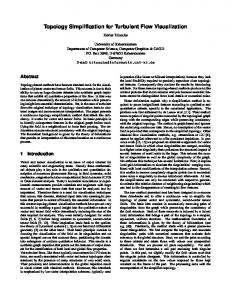
1 Introduction Multiresolution rendering involves rendering perceptually less significant objects in a scene at lower levels of detail and perceptually more significant objects at higher levels of detail. Most algorithms for creating multiresolution hierarchies of polyhedral objects [1, 2, 3, 4, 5, 6, 7, 8, 9, 10] preserve the topology of the input object. Preservation of the input topology is a desirable and sometimes even a crucial requirement of the end-application using the multiresolution hierarchy. For instance, information about the presence of tunnels and cavities in a molecule is quite important in biochemistry applications such as rational drug design. Regardless of the degree of surface simplification, it is crucial for these applications that such topological features be preserved. Similarly, adaptive simplifications for finite-element structures and study of fine tolerances between nearby parts in mechanical CAD requires the use of genus-preserving simplifications. However, in virtual environments one has to reconcile the mutually conflicting goals of visual realism and real-time interactivity. In such environments it often becomes necessary to relax the constraint of topology preservation in the interest of more aggressive simplification that yields faster rendering rates. For example, consider a mechanical part as shown in Fig. 1. As this part is moved away from the observer the holes and protuberances in the object will appear to become smaller, eventually reaching subpixel sizes. At such distances a topology-simplifying multiresolution hierarchy that simplifies away the holes is often preferable to a topology-preserving hierarchy that preserves the genus of an object, since 1
genus preservation comes at the cost of increased representation complexity. This paper addresses automatic creation of topology-simplifying multiresolution hierarchies.
(a)
(b) Figure 1: Topology simplifying multiresolution hierarchy Simplification of an object of arbitrary topological type can be viewed as a two-stage process – simplification of the topology (i.e. reduction of the genus) and simplification of the geometry (i.e. reduction of the number of vertices, edges, and faces). Our approach mainly addresses the former, although as we discuss in Section 4, it can also be used to a limited extent in removing small protuberances that fall in the latter category. In general, it is difficult for geometry-simplification techniques to remove small protuberances from models as cleanly and as naturally as our method (example Fig. 7). Although our approach is general and applicable to any polygonal dataset, we have developed a set of heuristics, presented in Section 3.3, that rapidly identify candidate regions for genus reductions. For a typical object there are few candidate regions for genus-reducing simplifications and this allows the running times for the genus-reducing stages to be usually much less as compared to the genus-preserving simplification stage. Our results demonstrate that genus reductions by small amounts can lead to large overall simplifications (Section 7). Details of our implementation are given in Section 6. One of the problems encountered in a large fraction of real-life CAD datasets are geometric degeneracies such as cracks. These geometric degeneracies arise from both human as well as computer-generated errors. Aside from leading to problems in manufacturability and simulation studies, data degeneracies result in visual artifacts in virtual environments. For instance, cracks cause light leaks in radiosity simulations and are also a leading cause behind unexpected shading discontinuities. In addition, they prevent the use of a large fraction of existing multiresolution hierarchy generation algorithms since most of them assume meshes with 2
no geometric degeneracies. Our approach can fill cracks that are narrower than a user-specified threshold �. We discuss this further in Section 5. The earlier conference-version of this paper [11] addresses exclusively the issue of controlled genus simplifications for polygonal models. In addition to more examples illustrating the results of our genussimplifying approach on CAD datasets, this paper also presents recent extensions of our research to deal with removal of protuberances based upon internal accessibility as well as repair of cracks often found in real-life mechanical CAD datasets.
2
Previous work
Our research builds upon previous work in three related but different areas of research – topology simplification of polygonal datasets, topology-varying reconstruction of surfaces, and repair of cracks in CAD models. The previous work in these areas is briefly surveyed next.
2.1
Topology-reducing Multiresolution Hierarchies
While there has been a significant amount of work done on creation of topology-preserving multiresolution hierarchies, much less attention has been focussed on creation of topology-simplifying hierarchies [7, 12, 13]. Rossignac and Borrel’s algorithm [7] subdivides the model by a global grid and uses a vertex clustering approach within each grid cell. All vertices that lie within a grid cell are combined and replaced by a new vertex. The polygonal mesh is suitably updated to reflect this. The nice properties of this approach are that it is quite fast and can work in presence of degeneracies often found in real-life polygonal datasets. This approach simplifies the genus if the desired simplification regions fall within a grid cell. However, it makes no guarantees about genus reduction and fine control over the genus simplification is not easy to achieve. He et al [12] present an algorithm to perform a controlled simplification of the genus of an object. It is a good approach that is applicable to volumetric objects on a voxel grid. It can handle degeneracies. However, since it works in the volumetric domain, polygonal objects have to be first voxelized. This often results in an increased complexity that is related to the volume of the object, not to its original representation complexity. Besides, the results from this approach lead to a scaled-down version of the simplified object that needs to be scaled back up to maintain the same size as the original object. This is not difficult but it adds another stage to the overall simplification process. Concurrent to our work on genus-reducing simplifications Schroeder [13] has defined vertex split and vertex merge operations on polygonal meshes for modifying the topology of polygonal models. This approach uses local distance criteria for geometry and topology simplification and achieves good results on large models. Like our method, this approach allows a fine control over the changes in the topology of an object. However, it does not identify and remove triangles that become internal after genus reductions and are thus no longer visible from the outside. Garland and Heckbert [14] present a quadric error metric that can be used to perform genus as well as geometric simplifications. The error at a vertex v is stored in the form a � symmetric matrix which can be used to compute the sum of squared distances of a given point with respect to the triangles adjacent to v . The algorithm proceeds by performing vertex-pair collapses and the error is accumulated from one vertex to the other by summing these matrices. The optimal position for a new vertex to replace a vertex-pair collapse is computed by solving a � linear system of equations. Popovi´c and Hoppe [15] introduce the operator of a generalized vertex split to represent progressive changes to the geometry as well as topology for triangulated geometric models. Progressive use of this operator results in representation of a geometric model as a progressive simplicial complex. They use an
4 4
4 4
3
error metric based upon Euclidean distance, surface discontinuities, local surface area, and mesh foldover penalties to prioritize amongst a candidate set of vertex pairs, obtained from a Delaunay triangulation of the model. Luebke and Erikson [16] use a scheme based on defining a tight octree over the vertices of the given model to generate hierarchical view-dependent simplifications. In a tight octree, each node of the octree is tightened to the smallest axis-aligned bounding cube that encloses the relevant vertices before subdividing further. If the screen-space projection of a given cell of an octree is too small, all the vertices in that cell are collapsed to one vertex and the parent cell is then considered for the same test. Adaptive refinement is performed analogously. This approach can accept input datasets with degeneracies. Luebke and Erikson’s approach can perform view-dependent genus simplification based on screen-space projection, polygon orientation as well as generate a user-specified triangle count approximation for a given view.
2.2
Topology-varying Surface Reconstruction
Much of previous work in surface reconstruction has focussed on reconstructing a surface of a single topological type. However, �-hulls allow one to generate a family of polyhedral objects with varying topology, as a function of an input parameter �, for a given set of points. Given a set of points P , a ball b of radius � is defined as an empty �-ball if b \ P �. For � � � 1, the �-hull of P is defined as the complement of the union of all empty �-balls [17, 18]. Three-dimensional �-shapes have been defined on the Delaunay tetrahedralization D of the input points P by Edelsbrunner and M¨ucke [19]. Let bT be the circumsphere of a k-simplex T and let its radius be �T . Let Gk;� ; � k � be the set of k-simplices 2 D for which bT is empty and �T < �. An �-complex of P , denoted by C� is the cell complex whose k-simplices are either in Gk;� or they bound the k -simplices of C�. The �-shape of P denoted by S� is the union of all simplices of C�. Thus, an �-shape of a set of points P is a subset of the Delaunay triangulation of P . Edelsbrunner [18], has extended the concept of �-shapes to deal with weighted points (i.e. spheres with possibly unequal radii) in three dimensions. An �-shape of a set of weighted points Pw is a subset of the regular triangulation of Pw . Recent work by Bernardini and Bajaj [20] uses �-hulls to deal with point-sets that represent a point sampling of mechanical CAD (polygonal or otherwise) models. Their work primarily deals with reconstruction of surfaces from unorganized sets of points, although it could potentially be used for genus-simplification of reconstructed surfaces if the input is either (a) a collection of unorganized set of points, or (b) a sampling of points from a given polygonal dataset. The existing work for �-hulls deals with only point- and sphere-based datasets. Our research extends the concept of �-hulls to polygonal datasets for performing genus-reducing simplifications. The primary targets of our research are the interactive three-dimensional graphics and visualization applications where topology can be sacrificed if (a) it does not directly impact the application underlying the visualization and (b) produces no visual artifacts. Both of these goals are easier to achieve if the simplification of the topology is finely controlled and has a sound mathematical basis. In Section 3 we outline our approach that has these properties.
=
�
0
1
3
( + 1)
2.3
Crack Repair in CAD Models
Real-life CAD models have several kinds of defects including coincident, intersecting, and incorrectly oriented polygons, T-junctions, T-edges, and cracks. Several researchers have addressed the problem of repairing cracks in CAD models. Barequet and Kumar [21] shift vertex positions using a heuristic based on area of the missing surface in merging two candidate edges of a crack. Murali and Funkhouser [22] adopt a solid-based approach in which they subdivide an imperfect model into a set of solid regions and then generate a correct triangulation enclosing the solid regions. Turk and Levoy [23] address the related issue of joining two polygonal meshes separated by a small 4
distance by clipping one with the other. Bøhn and Wozny [24] fill cracks by using local techniques. Baum et al. [25] handle the problem of cracks in meshes by grouping together vertices that are closer than a given value �. None of these methods can be easily generalized to be able to handle genus simplifications, whereas our approach can naturally correct cracks as well as generate genus-reducing simplifications. To be fair to the above methods, we would like to point out that several of them do more than just crack repair for CAD models, for example they consistently orient polygons, handle coincident polygons, and register multiple meshes; our approach cannot accomplish such general repair.
3
Genus simplification
The intuitive idea underlying our approach is to simplify the genus of a polygonal object by rolling a sphere of radius � over it and filling up all the regions that are not accessible to the sphere. This is the same as the underlying idea of �-hulls over point-sets. The problem of planning the motion of a sphere amidst polyhedral obstacles in three-dimensions has been very nicely worked out by Bajaj and Kim [26]. We use these ideas in our approach. Let us first assume that our polygonal dataset consists of only triangles; if not, we can triangulate the individual polygons [27, 28, 29]. Planning the motion of a sphere of radius �, say S � , amongst triangles is equivalent to planning the motion of a point amongst “grown” triangles. Mathematically, a grown triangle Ti � is the Minkowski sum of the original triangle ti with the sphere S � . Formally, Ti � ti � S � , where � denotes the Minkowski sum which is equivalent to the convolution operation. Thus, our problem reduces to efficiently and robustly computing the union of the S grown triangles Ti � . The boundary of this union, @ ni=1 Ti � , where n is the number of triangles in the dataset, will represent the locus of the center of the sphere as it is rolled in contact with one or more triangles and can be used to guide the genus simplification stage. We should point out here that our choice of the L1 metric over the L2 metric buys us robustness and efficiency but sacrifices the rotational invariance of error tolerance in the conventional Euclidean (L2 ) sense.
()
()
3.1
()= ()
() ()
()
Alpha prisms
()
We refer to an �-grown triangle Ti � as an �-prism. For general polygons, computing a constant radius offsetting is a difficult operation in which several degeneracies might arise [26]. However, for triangles this is an easy, robust, and constant-time operation. Computing the union of Ti � ; � i � n can be simplified by considering the offsetting operation in the L1 or the L1 metrics. This is equivalent to convolving the triangle ti with an oriented cube (which is the constant distance primitive in the L1 or the L1 metrics, just as a sphere is in the L2 metric). Offsetting a triangle ti in the L1 or the L1 metrics yields a Ti � that is a convex polyhedron (result of the convolution of an oriented cube with the triangle ti ). Example of a two-dimensional �-prism in the L1 distance metric is shown in Fig. 2. We choose the L1 distance metric over the L1 metric because the former results in axially-aligned unit-distance cubes, which are easier to deal with in union and intersection operations. We have efficiently implemented the construction of �-prisms for the L1 metric as outlined in Section 6.1.
( )1
()
3.2
Overview of our approach
Fig. 3 gives the overview of the stages involved. For clarity, the overview in the figure is given in two dimensions; extension to three dimensions (which we have implemented) is straightforward. Let us consider the behavior of our approach in the region of a two-dimensional “hole” abcde (shown unfilled). We first generate the �-prisms (Fig. 3(b)), compute their union (Fig. 3(c)), and generate a valid surface triangulation 5
(a)
(b)
Figure 2: (a) Triangle and L1 cubes (b) � prism
(a)
(b) Figure 3: Overview of the triangulation algorithm
(c)
from the union (Fig. 3(d)). The result of this process as shown for this example adds an extra triangle abe in the interior of the region abcde. This extra triangle is added in the region where the oriented L1 cube of side � could not pass through. S The computation of the union of the �-prisms, ni=1 Ti � , under the L1 metric is simply the union of n convex polyhedra. The union of n convex polyhedra can be computed from their pairwise intersections. Intersection of two convex polyhedra with p and q vertices can be accomplished in optimal time O p q [30]. A simpler algorithm to implement takes time O( p q p q ) [31]. With our approach one could, in principle, compute the union of �-prisms over the entire polygonal object (and not just along the boundary of the region of interest as shown in Fig. 3). This will result in automatic identification of the region abcde as being partially inaccessible to the L1 cube of side �, and therefore a candidate for getting filled. In practice, we have observed that the regions on an object that actually participate in simplification of the genus are few. As a result, a lot of effort is spent in processing those regions of the object that ultimately do not result in any simplifications. To avoid this extra computation and rapidly identify such regions that can be partially or completely triangulated we use a heuristic as outlined next.
2
()
)
( +
( + ) log( + )
2
3.3
Determination of tessellation regions
We define a tessellation region on an object as the region that is partially or completely inaccessible to an L1 cube of side �. A tessellation region is a closed-connected region bounded by a tessellation chain. A tessellation chain consists of a linear sequence of edges – the tessellation edges. In Fig. 3, the tessellation edges are fab; bc; cd; de; eag, the tessellation chain is abcdea , and the tessellation region is the unfilled
2
(
6
)
(
)
polygonal region abcde . There are three main stages in determination of the tessellation regions. We first determine the global set of tessellation edges that forms the boundaries of all the regions that need to be tessellated on an object. We next organize the tessellation edges into a set of tessellation chains. A tessellation chain is defined as a sequence of connected tessellation edges whose every vertex is adjacent to exactly two tessellation edges, except the first and the last vertices which can have a different degree of tessellation edges. The third stage involves orienting each tessellation chain so that the tessellation region lies on its left side (assuming that the polygons are oriented counterclockwise). Determination of tessellation edges In principle, it is possible to determine all tessellation regions (and hence tessellation edges) from the union of �-prisms over the entire polygonal object. However, this is rather slow and we have observed that in practice for most mechanical CAD models the genus-reducing simplifications occur in well-defined regions. To efficiently determine the tessellation edges we currently use the heuristic that genus-reducing simplifications usually occur in the neighborhood of sharp edges. We define a sharp edge to be one for which the dihedral angle between the neighboring triangles is greater than 0. We have found this to be a good heuristic for some threshold ; we currently use the constant mechanical CAD models.
= 70
Determination of tessellation chains After we have determined the tessellation edges, they are initially stored as an edge soup – an unorganized collection of edges. We organize the tessellation edges into tessellation chains by using a linear-time depth-first scanning strategy. At the end of this stage we have tessellation chains as shown in Fig. 4.
Figure 4: Tessellation chains
Orienting tessellation chains For each tessellation chain we need to determine the side on which the tessellation region will lie. Once this side has been determined, we orient the tessellation chain such that the tessellation region lies on its left. If we were to use the global information from a completely computed �-hull of the polygonal object, determination of the orientation would be quite easy, although expensive. To speed-up this stage, we use the heuristic that the tessellation regions have a larger variation of the surface normal. This heuristic works quite well for mechanical CAD models for which almost all genus-reducing simplifications occur in holes, tunnels, or sharp concavities in regions that are otherwise flat. Orientation of the tessellation chains helps in tiling as well as removal of the internal triangles as discussed next.
7
3.4
Generating a valid surface triangulation
S
()
We consider those vertices ui of the union of �-prisms, ni=1 Ti � , that belong to two or more �-prisms. For each vertex ui , we consider every pair of �-prisms Tj � and Tk � to which ui belongs. If we center the L1 cube of side � at ui , it will touch two edges (say el and em ), one from each triangle tj and tk . Let the edge el vl0 ; vl1 , and the edge em vm0 ; vm1 For example in Fig. 3, ui g1 , el ab, and em ae. If the L1 cube of side � centered at the point ui contains a pair of non-adjacent vertices vp and vq out of fvl0 ; vl1 ; vm0 ; vm1 g (in this example, vertices b and e), then we add the edge vp; vq (in this example, we add edge be) to the set of diagonal edges that will be used to generate the surface triangulation. In this example if the L1 cube at g1 did not contain either of the vertices b or e, we would not have added any diagonal edge. At the end of this stage we have the superset of the diagonals required for the final triangulation as well as a collection of oriented tessellation chains. The diagonals and the oriented tessellation chains are used in the surface reconstruction approach as outlined in [32]. The objective function that we use for optimization in the surface reconstruction is minimizing the length of the diagonal edges used (shortest edge first). This gives us a unique and consistent triangulation. As a result of our triangulation above, some triangles that were initially on the surface of the object now become interior as shown in Fig. 5. We identify and remove the internal triangles as follows. All the tessellation regions that we covered have oriented tessellation boundaries. Walking along the direction of the tessellation chain, we classify the left side as interior (i.e. the region that has just been covered) and the right side as exterior (this assumes counter-clockwise orientation of polygons). We start from a triangle belonging to the input object that lies to the left (i.e. the interior) of an oriented tessellation chain and spread out in a breadth-first manner until we hit one of the hole edges or another triangle that has been similarly traversed. All triangles that are thus traversed are marked as interior and eliminated. In Fig. 5(c) the patched triangles are shown in green and the interior triangles that are eliminated are shown in yellow.
=
=(
(a)
2
)
() )
=(
2
()
=
(
(b)
(c)
= )
(d)
Figure 5: Overview of the genus-reducing simplification
4 Removal of Protuberances Current geometry-based simplification techniques are based on the local geometric properties such as curvature and distance along the local normal. Most of these techniques do not take the gross shape of the object into account. Alpha-hulls have been used in the past to define the shape of a set of unorganized points [17]. Our approach that is based on a three-dimensional variant of �-shapes is consequently well-suited to working on the problem of identifying and simplifying small protuberances and features. Let us reconsider the concept of �-hulls in three dimensions. If we ignore the internal cavities, the �-hull for a set of points intuitively corresponds to the surface defined by a sphere of radius � as it is rolled around 8
0
the points. When the value of � is , the �-hull is simply the collection of the input points. As the value of � is increased, more and more points get connected to each other. With an increasing value of � the regions of concavities in the external surface get progressively ”filled”. Finally, when � 1, all concavities in the external surface are filled and the alpha-hull is the convex hull of the input points. This is the basic idea behind our approach to fill up holes and regions of sharp concavities for polygonal models.
=
(a)
(b)
(c)
(d)
(e)
(f)
Figure 6: Simplification of protuberances In several finite-element applications where approximations to the original model are acceptable it is important to remove small protuberances from the input model without changing the surrounding geometry too much. In virtual environments too, it may be important to be able to remove such small-scale features without affecting their neighborhood to get a better approximation to the overall shape. As an example consider the object in Fig. 6(a). A local-geometry-based approach might simplify it to an object as shown in Fig. 6(b). However, what might be more desirable in certain situations is the object represented in Fig. 6(f). We have observed that we can very easily extend our code to simplify away the protuberances by simply moving the L1 cube on the interior of the object as opposed to the exterior. The protuberances on the outside of the object look like concavities from the inside. Therefore just as our approach looking at an object from the outside fills-up the concavities, holes, and tunnels, it should be able to simplify away the protuberances if we considered the object from inside. We have tried this and it works very nicely. This is illustrated in Fig. 6 for the case of the L2 primitive – a sphere. Figs. 6(c), (d) show the results of rolling the sphere on the exterior of the object and the identification and removal of concavities. Figs. 6(e), (f) show the results of rolling the sphere on the interior of the object and the identification and removal of protuberances. As far as the implementation is concerned, the rolling of a L2 sphere or L1 cube on the interior as opposed to the exterior is accomplished by simply flipping (inverting) the normals of every triangle in the polygonal model to conceptually turn the object inside-out. 9
(a) Original 612 triangles
(b) Protuberance 12 triangles
(c) Edge collapse 120 triangles
Figure 7: Comparing protuberance simplification with edge collapse Fig. 7(c) shows the results of a topology-preserving edge collapse algorithm for the same error tolerance as used in Fig. 7(b). The reason why the model in Fig. 7(c) did not simplify any further is similar to the reason why genus-simplifications allow better overall simplifications, which is that the topology-preserving simplifications block simplifications by not allowing creation of non-manifold edges (i.e. edges that share three triangles) and vertices. This led us to explore if we could extend our genus-simplifying approach to be able to remove protuberances.
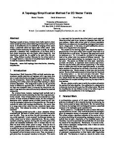
5 Repair of Cracks Cracks arise in CAD models due to both human as well as computer-generated errors. Some of the reasons underlying these errors are: (a) too much time is required to correct or avoid all cracks and draftsmen working on large projects under deadline pressures resort to various shortcuts, and (b) tessellation algorithms during CSG boolean operations by commercial modelers on curved surfaces often yield cracks due to improper handling of singularities. Cracks cause several problems in the computer graphics pipeline. In global illumination computations cracks cause distracting light leaks. Cracks also cause artifacts such as shading discontinuities and aliasing. Algorithms that convert triangular meshes to triangle-strips terminate prematurely at cracks leading to suboptimal conversions. A large number of multiresolution hierarchy creation algorithms which rely on the local geometry information fail to work with such cracks. Our work on simplification of the genus extends naturally to handling of cracks in real-life polygonal datasets. We have tested our implementation on several meshes with cracks and missing triangles and have achieved encouraging results. An example CAD object is shown in Fig. 8. Most commercial radiosity packages currently compute the radiosity solution on a per-polygon basis leaving topological cracks where two polygons meet. An example showing crack repair for the mesh generated by a commercial radiosity package is shown in Figure 9. In our implementation, all one-sided edges (i.e. edges that have only one adjacent triangle) are currently assumed to be candidate edges for defining a 10
(a) 456 triangles
(b) 66 triangles
Figure 8: Crack repair for an industrial CAD part
(a) Radiositized dataset
(b) Cracks in underlying mesh
(c) Repaired mesh
Figure 9: Crack repair for radiosity dataset crack and are considered as tessellation edges for further processing. Most of the processing for cracks is similar to the processing for genus simplifications. This is useful in that it allows us to handle cracks as a special case of genus simplification. To speed up the processing for cracks we have implemented a few differences from the case for genus simplification. In our current implementation for genus-simplifications we define the tessellation edges and tessellation regions based on a heuristic (Section 3.3). However, our definition of the tessellation edges and tessellation regions for the cracks is clearly accurate and not a heuristic. For the case of cracks, unlike for genus simplification, we do not need to remove any internal triangles left after patching over the crack. As a quick overview, �-prisms are constructed around the crack edges just as they are around any other tessellation edges. The union of the �-prisms is used for defining the candidate diagonals and these are then used for generating a valid triangulation. Thus, we fix cracks by adding extra triangles to the surface. Some of the triangles that we add may be long and skinny. For example, a T-junction crack is fixed by adding a degenerate triangle. These are appropriately handled during the geometry simplification stages.
6 6.1
Implementation details Efficiently constructing alpha prisms
2
The �-prism is the convex hull of the three axially aligned L1 cubes, each of side � units, centered at each of the three vertices of a triangle. There are several sets of coplanar points for this case and as a result the traditional methods of computing convex hulls do not work robustly here. One solution to this robustness problem is to perform perturbation of all the input points [33, 34]. Although such approaches
11
guarantee removal of all degeneracies, they require multi-precision arithmetic which is slow. Besides, such perturbations lead to generation of unnecessary sliver triangles in the union of the �-prisms. To overcome these limitations, we decided to adopt a different, although specialized, approach That works quite efficiently and robustly. We next outline the basic idea of this approach. 0001
0001
0000 1000
0000
1000
0000
0000 0000
1000
0001
0000
0000
0000
0000
0000
0000
0100
0000
0100
0000
0010
0010
0110
Figure 10: Fast computation of alpha prisms We associate a 6-bit vector with each vertex, edge, and face of the three L1 cubes. Each of the six bits of the bit-vector associated with a vertex v is if and only if the corresponding property holds amongst all of the vertices : fminimum x, maximum x, minimum y, maximum y, minimum z, maximum zg. Thus, bit[0] of a vertex will be if its x-coordinate has the minimum value amongst all the vertices; it will be otherwise. The edge bit-vector is computed as the logical bit-wise AND of its two vertices’ bit-vectors. The face bit-vector is the logical bit-wise AND of its four edges’ bit-vectors. The �-prism can be computed by using the information from these vertex, edge, and face bit-vectors. For instance, all the cubes’ faces that have non-zero bit-vectors belong to the �-prism. Details of this approach are outside the scope of this paper; they will be described elsewhere. The computation of the �-prism using this strategy for the twodimensional case (where we use 4-bit vectors) is shown in Fig. 10. Notice that only those edges of the L1 squares that have non-zero bit-vectors are a part of the two-dimensional �-prism (analogous to the faces of the L1 cubes in three dimensions).
24
0
6.2
1
1
24
Efficiently intersecting alpha prisms
The �-neighborhood of a triangle ti is defined as the set of all triangles tj such that the intersection of their T �-prisms is non-null, Ti � Tj � 6 �. Every such pair of �-prisms is defined to be �-close to each other. The first stage in generating a valid surface triangulation is to identify the pairs of �-prisms that are �-close to each other. For practical values of �, which are relatively small, the average size of the �-neighborhood of a triangle has been empirically observed to be a small constant. We use a global grid to speed up the determination of the �-neighborhood for each triangle ti . Each side of the cubical grid is � units, to minimize the number of neighboring cubes that have to be considered for determining the �-neighborhood of a given triangle. The �-prisms’ intersection calculation is based on a face-by-face intersection procedure. To compute the union of N �-prisms, we start with the first prism and at ith step ( � i � N ) we compute the union of the ith �-prism with the currently computed union of to i , �-prisms. This procedure reduces the total number of intersection computations since it avoids considering those faces that are in the interior of the union of �-prisms at the ith stage.
()
( )=
2
1
12
1
2
7
Results and discussion
We have implemented the approach outlined above and have obtained very encouraging results. We ran our implementation on one R10000 processor of SGI Challenge for all the results reported here. The various mechanical parts on which we tested our algorithm and reported our results are shown in Figs. 1, 11 – 13. An example of a multiple levels-of-detail hierarchy can be seen in Fig. 11. Here the object complexity was reduced as follows: (a) original object had 756 triangles; (b), (c): genus reduction removed the two holes on the side and followed this by geometry simplification, (d), (e): a second-level genus-preserving simplification removed a hole at the top and followed by a geometry reduction to yield a final object (f) with 298 triangles. Our results for higher polygon-count objects appear in Figs. 12 and 13.
(a) 756 triangles
(b)
(c)
(d) (e) (f) 298 triangles Figure 11: Alternating genus-preserving and genus-reducing simplifications We chose the Simplification Envelopes [1] approach to perform our genus-preserving simplifications. All error tolerances (� and �) given in this section are specified as the percentage of the diagonal of the bounding box of the object. We first simplified the given objects using the genus-preserving approach with a tolerance of �. Then on this simplified object we compared the results of the following two simplification strategies: (a) genus-reducing simplifications with a tolerance of � followed by genus-preserving simplifications with a tolerance of � (b) genus-preserving simplifications with a tolerance of �
+�
The results of our comparisons are given in Table 1. As can be seen, performing genus-reducing simplification with genus-preserving simplifications vastly improves the overall simplification ratio. The timings in the following table are in units of seconds, minutes, and hours and are accordingly marked by s, m, and h, respectively. Not only did we observe the genus-reducing simplifications improved the overall simplification ratio substantially, we also observed that the times taken by the genus-reducing stage were reasonably small. This is partly because of our use of heuristics as given in Section 3.3 which we have observed work quite well for mechanical CAD datasets. 13
(a) 74,168 triangles
(b) 7,486 triangles
Figure 12: Wire-ways from a notional submarine
(a) 158,728 triangles
(b) 2216 triangles
Figure 13: Batteries of a notional submarine
14
Original Object Name Num Tris Box Sphere Block Wireways Fixture Batteries
1612 2058 17644 74168 74396 158728
� 1.0 5.5 0.4 0.01 0.3 0.005
Genus-Preserving Simplification Time Num Tris 30 s 100 s 24 m 34 m 5:30 h 42 m
166 432 2054 69612 10806 126220
Genus-Reducing and Genus-Preserving Simplification Genus Genus Num Reducing Preserving Tris Time Time 2.0 0.3 s 1.0 2.0 s 14 11.0 0.3 s 5.5 7.3 s 136 0.8 5.6 s 0.4 20 s 78 0.01 20 s 0.03 15 m 7486 0.6 129 s 0.3 42 s 62 0.005 13.8 s 0.01 5.2 m 2216
�
�
� +
�
3.0 16.5 1.2 0.05 0.9 0.015
Genus-Preserving Simplification Time Num Tris 4.2 s 19.2 s 280 s 23.4 m 11:22 h 28.5 m
138 162 1622 38400 7300 124806
Ratio of Simplifcation Improvement 9.86 1.19 20.79 5.12 117.7 56.32
Table 1: Results of genus-reducing and genus-preserving simplifications The figures for block and fixture can be seen in the conference-version of this paper [11]. Batteries from the Auxiliary Machine Room dataset of a notional submarine from Electric Boat Corporation are shown in Figs. 14, 7, and 13. Wireways model consists of hollow tubes that contain the wiring for the notional submarine model from Electric Boat Corporation and appear in Fig. 12.
(a) 612 triangles
(b)
(c)
(d)
(e)
(f) 12 triangles
Figure 14: Alternating geometry and protuberance simplifications As can be seen from Table 1 and the accompanying figures, our approach indicates promising results for genus reduction, protuberance simplification, and crack repair. Using our approach for genus-reductions and protuberance simplifications with traditional geometry simplification techniques we have been able to achieve significant simplification factors over what genus-preserving geometry simplifications alone could accomplish.
15
8
Conclusions and future work
We have presented an approach that performs a controlled simplification of the genus of polygonal objects. This approach works quite well in conjunction with the traditional genus-preserving simplification approaches and yields substantially lower representation complexity objects than otherwise possible. Our approach can work in presence of limited kinds of degeneracies, such as T-junctions and T-edges, that are quite widespread in real-life mechanical CAD datasets. Our approach is easily extensible to be able to simplify away small protuberances and repair cracks in CAD models. Currently we only use the size of the cross-section of the protuberance for removing it. Further work needs to be done to examine other criteria such as area and/or volume of the protuberances. We currently use heuristics that rapidly detect holes and other cavities commonly found in CAD models. We plan to further explore other heuristics that will rapidly determine the tessellation regions on other kinds of scientific visualization datasets. Our approach currently works only for polygonal objects. Its generalization to objects described by higher-order algebraic patches will be an interesting area for future work. Our approach does not at present handle certain degeneracies such as coincident polygons, self-intersecting meshes, and meshes with inconsistent orientations of polygons. Alpha hulls have been shown to work quite well for reconstructing surfaces from unorganized collections of points. It should be possible to extend the current work and merge it with that line of research to be able to handle the above degeneracies as well. Our approach is based upon the concept � hulls which have in the past been found to be useful in determining the accessibilities. This raises the possibility of extending our approach to be able to do the preprocessing required for other accessibility-based graphics algorithms such as accessibility shading [35].
Acknowledgements The first author has been supported by a Fulbright/Israeli Arab Scholarship. This work has been supported in part by the Honda Intiation Grant and the National Science Foundation CAREER award CCR-9502239. The CAD objects used in this paper are a part of the dataset of a notional submarine provided to us by the Electric Boat Corporation. We would like to acknowledge LightWork Design Ltd. for supplying the radiosity dataset used for Figure 9. The radiosity solution for that image was generated using LightWorks Pro.
References [1] J. Cohen, A. Varshney, D. Manocha, G. Turk, H. Weber, P. Agarwal, F. P. Brooks, Jr., and W. V. Wright, “Simplification envelopes,” in Proceedings of SIGGRAPH ’96 (New Orleans, LA, August 4–9, 1996). ACM SIGGRAPH, August 1996, Computer Graphics Proceedings, Annual Conference Series, pp. 119 – 128, ACM Press. [2] T. D. DeRose, M. Lounsbery, and J. Warren, “Multiresolution analysis for surface of arbitrary topological type,” Report 93-10-05, Department of Computer Science, University of Washington, Seattle, WA, 1993. [3] A. Gu´eziec, “Surface simplification with variable tolerance,” in Proceedings of the Second International Symposium on Medical Robotics and Computer Assisted Surgery, MRCAS ’95, 1995. [4] B. Hamann, “A data reduction scheme for triangulated surfaces,” Computer Aided Geometric Design, vol. 11, pp. 197–214, 1994. 16
[5] H. Hoppe, “Progressive meshes,” in Proceedings of SIGGRAPH ’96 (New Orleans, LA, August 4–9, 1996). ACM SIGGRAPH, August 1996, Computer Graphics Proceedings, Annual Conference Series, pp. 99 – 108, ACM Press. [6] H. Hoppe, “View-dependent refinement of progressive meshes,” in Proceedings of SIGGRAPH ’97 (Los Angeles, CA). ACM SIGGRAPH, August 1997, Computer Graphics Proceedings, Annual Conference Series, pp. 189 – 197, ACM Press. [7] J. Rossignac and P. Borrel, “Multi-resolution 3D approximations for rendering,” in Modeling in Computer Graphics. June–July 1993, pp. 455–465, Springer-Verlag. [8] W. J. Schroeder, J. A. Zarge, and W. E. Lorensen, “Decimation of triangle meshes,” in Computer Graphics: Proceedings SIGGRAPH ’92. ACM SIGGRAPH, 1992, vol. 26, No. 2, pp. 65–70. [9] G. Turk, “Re-tiling polygonal surfaces,” in Computer Graphics: Proceedings SIGGRAPH ’92. ACM SIGGRAPH, 1992, vol. 26, No. 2, pp. 55–64. [10] J. Xia, J. El-Sana, and A. Varshney, “Adaptive real-time level-of-detail-based rendering for polygonal models,” IEEE Transactions on Visualization and Computer Graphics, vol. 3, No. 2, pp. 171 – 183, June 1997. [11] J. El-Sana and A. Varshney, “Controlled simplification of genus for polygonal models,” in IEEE Visualization ’97 Proceedings. October 1997, pp. 403 – 410, ACM/SIGGRAPH Press. [12] T. He, L. Hong, A. Varshney, and S. Wang, “Controlled topology simplification,” IEEE Transactions on Visualization and Computer Graphics, vol. 2, no. 2, pp. 171–184, June 1996. [13] W. Schroeder, “A topology modifying progressive decimation algorithm,” in IEEE Visualization ’97 Proceedings. October 1997, pp. 205 – 212, ACM/SIGGRAPH Press. [14] M. Garland and P. Heckbert, “Surface simplification using quadric error metrics,” in Proceedings of SIGGRAPH ’97 (Los Angeles, CA). ACM SIGGRAPH, August 1997, Computer Graphics Proceedings, Annual Conference Series, pp. 209 – 216, ACM Press. [15] J. Popovi´c and H. Hoppe, “Progressive simplicial complexes,” in Proceedings of SIGGRAPH ’97 (Los Angeles, CA). ACM SIGGRAPH, August 1997, Computer Graphics Proceedings, Annual Conference Series, pp. 217 – 224, ACM Press. [16] D. Luebke and C. Erikson, “View-dependent simplification of arbitrary polygonal environments,” in Proceedings of SIGGRAPH ’97 (Los Angeles, CA). ACM SIGGRAPH, August 1997, Computer Graphics Proceedings, Annual Conference Series, pp. 198 – 208, ACM Press. [17] H. Edelsbrunner, D. G. Kirkpatrick, and R. Seidel, “On the shape of a set of points in the plane,” IEEE Transactions on Information Theory, vol. IT-29, no. 4, pp. 551–559, July 1983. [18] H. Edelsbrunner, “Weighted alpha shapes,” Tech. Rep. UIUCDCS-R-92-1760, Department of Computer Science, University of Illinois at Urbana-Champaign, 1992. [19] H. Edelsbrunner and E. P. M¨ucke, “Three-dimensional alpha shapes,” ACM Transactions on Graphics, vol. 13, no. 1, pp. 43–72, January 1994. [20] F. Bernardini and C. Bajaj, “Sampling and reconstructing manifolds using alpha-shapes,” Tech. Rep. CSD-97-013, Department of Computer Sciences, Purdue University, 1997. 17
[21] G. Barequet and S. Kumar, “Repairing cad models,” in IEEE Visualization ’97 Proceedings. October 1997, pp. 363 – 370, ACM/SIGGRAPH Press. [22] T. M. Murali and T. A. Funkhouser, “Consistent solid and boundary representation from arbitrary polygonal data,” in Proceedings, 1997 Symposium on Interactive 3D Graphics, 1997, pp. 155 – 162. [23] Greg Turk and Marc Levoy, “Zippered polygon meshes from range images,” in Proceedings of SIGGRAPH ’94 (Orlando, Florida, July 24–29, 1994), Andrew Glassner, Ed. ACM SIGGRAPH, July 1994, Computer Graphics Proceedings, Annual Conference Series, pp. 311–318, ACM Press, ISBN 0-89791-667-0. [24] J. H. Bøhn and M. J. Wozny, “A topology based approach for shell closure,” in Geometric Modeling for Product Realization, M. J. Wozny P. R. Wilson and M. J. Pratt, Eds., pp. 297–319. North Holland, Amsterdam, 1993. [25] D. R. Baum, Mann S., Smith K. P., and Winget J. M., “Making radiosity usable: Automatic preprocessing and meshing techniques for the generation of accurate radiosity solutions,” Computer Graphics: Proceedings of SIGGRAPH’91, vol. 25, No. 4, pp. 51–60, 1991. [26] C. Bajaj and M.-S. Kim, “Generation of configuration space obstacles: the case of a moving sphere,” IEEE Journal of Robotics and Automation, vol. 4, No. 1, pp. 94–99, February 1988. [27] R. Seidel, “A simple and fast incremental randomized algorithm for computing trapezoidal decompositions and for triangulating polygons,” Comput. Geom. Theory Appl., vol. 1, pp. 51–64, 1991. [28] K. Clarkson, R. E. Tarjan, and C. J. Van Wyk, “A fast Las Vegas algorithm for triangulating a simple polygon,” Discrete Comput. Geom., vol. 4, pp. 423–432, 1989. [29] A. Narkhede and D. Manocha, “Fast polygon triangulation based on seidel’s algorithm,” Graphics Gems 5, pp. 394–397, 1995. [30] B. Chazelle, “An optimal algorithm for intersecting three-dimensional convex polyhedra,” SIAM J. Comput., vol. 21, no. 4, pp. 671–696, 1992. [31] D. E. Muller and F. P. Preparata, “Finding the intersection of two convex polyhedra,” Theoret. Comput. Sci., vol. 7, pp. 217–236, 1978. [32] H. Fuchs, Z. M. Kedem, and S. P. Uselton, “Optimal surface reconstruction from planar contours,” Commun. ACM, vol. 20, pp. 693–702, 1977. [33] H. Edelsbrunner and E. P. M¨ucke, “Simulation of simplicity: a technique to cope with degenerate cases in geometric algorithms,” in Proc. 4th Annu. ACM Sympos. Comput. Geom., 1988, pp. 118–133. [34] I. Emiris and J. Canny, “An efficient approach to removing geometric degeneracies,” in Eighth Annual Symposium on Computational Geometry, Berlin, Germany, June 1992, ACM Press, pp. 74–82. [35] G. Miller, “Efficient algorithms for local and global accessibility shading,” in Proceedings of SIGGRAPH 94 (Orlando, Florida, July 24–29, 1994). July 1994, Computer Graphics Proceedings, Annual Conference Series, pp. 319–326, ACM SIGGRAPH.
18