network resource management in the context of a central- ized sensor rate selection mechanism for an event detection application scenario. 1. INTRODUCTION.
Toward Quality of Information Aware Rate Control for Sensor Networks Zainul Charbiwala, Sadaf Zahedi, Younghun Kim, Mani B. Srivastava Dept. of Electrical Engineering University of California, Los Angeles
ABSTRACT In sensor networks, it is the Quality of Information (QoI) delivered to the end user that is of primary interest. In general, measurements from different sensor nodes do not contribute equally to the QoI because of differing sensing modalities, node locations, noise levels, sensing channel conditions, fault status, and physical process dynamics. In addition, metrics of QoI are highly application dependent, such as probability of detection of an event or fidelity of reconstruction of a spatio-temporal process. Despite these considerations, traditional data dissemination protocols in sensor networks have been designed with a focus on metrics such as throughput, packet delivery ratio, latency, and fair division of bandwidth, and are thus oblivious to the importance and quality of sensor data and the target application. In this paper, we argue for sensor network protocols that are cognizant of and use feedback from the sensor fusion algorithms to explicitly optimize for application-relevant QoI metrics during network resource allocation decisions. Through analysis and simulation we demonstrate the application-level performance benefits accruing from such a QoI-aware approach to network resource management in the context of a centralized sensor rate selection mechanism for an event detection application scenario.
1.
INTRODUCTION
Wirelessly networked sensors are now routinely being used in experiments that further our understanding of the natural world and for the estimation and detection of various events within it. In the first case, a key metric of performance is the fidelity with which a spatio-temporal phenomenon is recovered, while in the second, it is reliable detection that is important. In both scenarios, designers strive to ensure that the highest quality data is extracted from the network and it would seem intuitive then, that these metrics should somehow be considered within the data collection process. However, designs for network services in sensor networks have traditionally focused on lower layer metrics such as throughput (or goodput) and fairness [1] and do not capture application-relevant objectives adequately. In this paper, we argue that application-level feedback is especially important for network protocol design in sensor networks. The motivation for meticulous sensor placement is similar – exploiting application layer domain knowledge while positioning sensors can provide the same information with a fraction of the nodes. Early sensor network research envisioned sensors being deployed, for the most part, in an ad-hoc fashion, requiring estimation from randomly (or uni-
Young H. Cho The Computer Network Division University of Southern California Information Sciences Institute
formly) placed sensors. However, many environmental phenomena vary slowly as a function of space and samples at locations close by are often correlated. By explicitly constructing statistical models of the phenomena, researchers are able to better predict locations that will either maximize the collective entropy or, even better, reduce the entropy at the unselected positions. For some experiments, this technique has led to a 5x [2] reduction in node density. Considering, in particular, the networking stack, numerous works have focused on special medium access protocols for sensor networks. The key argument made in favor of the specialist methodology is that by utilizing apriori knowledge of the traffic model, the energy drain due to always-on radio receivers can be effectively mitigated ([3], etc.). Designs using this guideline have shown tremendous improvements in network lifetime and are hence regularly used in real deployments ([4]§3.2.3). Similarly, some routing protocols [5] leverage the fact that sensing applications typically involve distributed data collection followed by centralized processing and therefore a tree topology with the fusion center at the root is adequate. In the same vein, designers of transport protocols [6] have utilized the fact that flows in sensor network applications can be made mutually non-interfering through cooperative scheduling, leading to a simplified design and conditionally high throughput. However, transport protocols have maintained that “all bits are created equal” and thus data from different source nodes are handled equitably within the network. For traffic engineering in computer networks, researchers introduced the concept of Quality of Service (QoS) as a means of labeling and prioritizing data flows according to a set of static predefined policies to ensure that data from the most important source or flow gets delivered (first). For sensor networks, however, this definition of QoS is inadequate because the notion of importance is associated not with a source, but with the data itself and moreover, on the value of the data to the end user of the application. One may interpret this as saying that the importance of a source node and its resultant share of network resources should now depend on the quality of data currently being produced (sensed) by the node. This requires a form of dynamic QoS that translates the value of data from a node to its priority on-the-fly. We dub this “value of sensed data” the Quality of Information (QoI) and in this paper, we illustrate a mechanism of quantifying and utilizing QoI for allocating network resources at the transport protocol layer. Computing a measure of QoI for a node is hard since it is affected by multiple factors that include its location, its sensing modalities, am-
bient noise levels, sensing channel conditions, fault status, and physical process dynamics, all of which may vary temporally. Instead, we propose to directly use feedback from the sensor fusion algorithms in an effort to capture these effects holistically on the application itself. Before delving into a case study detailing the use of QoI (§3), we attempt to develop an intuitive appreciation of this concept.
1.1
1.2
The contributions of this work are threefold: • We introduce a notion of QoI that quantifies the value of data sensed at a node by observing feedback from the sensor fusion algorithm. • We exemplify the employment of this tool to network resource management in the context of a centralized sensor rate selection mechanism for an event detection application scenario.
Foveated Sensing
Consider the following example: we wish to track a moving target in a field. The field is instrumented with a set of acoustic sensors [7] for animal tracking, say. To improve tracking accuracy a heuristic could be applied: once a target is detected and is being actively tracked, nodes closer to the target should be able to send more data than ones further away from it. Intuitively, one would expect that nodes closer to the event have access to better quality data and funneling more data from these nodes would improve the accuracy at the fusion center. Conversely, dropping data from distant nodes under congestion would not affect the end result significantly. This scheme is depicted pictorially in Figure 1. In effect, the heuristic dynamically changes the priority of nodes’ transmissions based on an estimate of the event location (one could go further to predict direction and preemptively control rates as well). A mechanism akin to this, termed foveated sensing, occurs in the human vision system to focus our attention on the most salient objects in our field of view [8]. In this case, we could imagine that a node’s QoI is higher if it closer to a target, but in general QoI would depend on the end goal of the application. Formally, we may define QoI as an application dependent objective function that has a monotonic relationship to the accuracy of the final inference. For example, a good QoI metric for an event detection scenario would be the probability of error (Pe ), since it is considered a primary performance benchmark for this application. We posit, thus, that adapting our network protocols to make Pe a first-class citizen would result in more efficient network operation. Practically, however, computing error probability explicitly requires ground truth. Instead, we use confidence measures provided by sensor fusion algorithms as a proxy for QoI feedback. We also show in §3.1 how Pe can be approximately computed for special cases. Note that by this argument, neither throughput nor fairness are valid QoI metrics. Increased throughput (more data reaching the fusion center) may come at the cost of some nodes being unable to transmit, while fairness may prevent the ‘right’ nodes from transmitting at higher rates. On the other hand, a QoI aware approach ensures that the best nodes communicate their information, while unimportant ones are curtailed from clogging the network. This conclusion is studied in more detail in §4.
Figure 1: An example of foveated sensing. Sensors (dots) closer to the event (blue star) send out more data (darker shades) than ones further away.
Contributions and Assumptions
• We demonstrate the application-level performance benefits accruing from such a QoI-aware approach and evaluate the costs incurred in adding feedback traffic from the sensor fusion algorithm. We should also clarify that this paper describes early work towards identifying objectives that better capture the intent of the transport protocol designer and is not intended as a blue print for a rate control protocol. Also, in order to form an end-to-end argument, we require to make assumptions that simplify our analysis. In particular, we assume that the wireless medium is centrally scheduled so that there is no channel contention and that the fusion center has complete route information to all nodes in the network. Before we delve into details of our problem formulation in §3, we describe some work related to our own.
2.
RELATED WORK
The use of the term QoI is a relatively recent development [9] but much research has been previously conducted for making protocols application-aware under the umbrella of cross-layer design [10, 11]. There have even been works specifically targeted towards sensor networks [12, 13], the main motivation behind which, is improving the lifetime of these extremely energy constrained devices. Our philosophy toward a QoI aware approach is similar in vein but provides a more general framework that can be applied to any objective of interest, or a weighted combination of multiple objectives. The following text lists specific examples that are particularly relevant to our approach. Gelenbe, et al. [14] explored routing mechanisms that provide differential service to low-priority high-volume routine sensor measurements and high-priority low-volume unusual event reports by adaptively dispersing the routine traffic to secondary paths so that the event reports can be sent through faster paths with better delay characteristics. For rate control algorithms for sensor networks, Rangwala, et al. (IFRC [15]) developed many of the fundamental blocks required to implement a functional protocol. They established a systematic model for flow interference and evolved mechanisms to detect and circumvent it. Later, Kim, et al [6] and Paek, et al. [16] presented Flush and RCRT respectively. Flush is tailored toward reliable bulk transfers and is fully distributed while RCRT transports sensor data reliably from many sources using end-to-end explicit loss recovery, placing rate adaptation functionality at the sinks and resulting in higher efficiency and flexibility. Our approach is similar to that of RCRT in that it exploits a centralized view of the network, but differs in the end objective. Chen, et al [1] describe a technique that achieves optimal maxmin fair rate assignments using an iterative linear programming approach. We implement a similar approach to
compare our QoI-aware technique to maxmin fairness. Finally, Fan et al. [17] recently presented optimal maxmin fair schemes for energy harvesting nodes. Though, we do not yet consider nodes’ energy conditions within our problem framework, we show how additional constraints could be incorporated easily.
3.
PROBLEM FORMULATION
In this section, we construct block-by-block a centralized rate control mechanism for an event detection scenario. In essence, we would like to control sensing and transmission rates for each node from a fusion center that has access to feedback from the sensor fusion algorithm. We could paraphrase this goal as: To optimize rate allocation with respect to a tractable Quality of Information metric for transport of sensor measurements in a multi-node multi-hop network with a centralized fusion algorithm.
3.1
Error Probability as a QoI Metric
In a detection scenario, key performance metrics are the probability of false positives (false alarms) and false negatives (missed detections). Minimizing a union of these, termed error probability (Pe ) would result in optimal performance. Since we know that network capacity is bounded, nodes may need to curtail the amount of information they send to the fusion center. The question is: How is Pe affected by the transmission rate from each node? This is hard to answer in general, but can be attempted with a specific scenario. Consider a centralized multi-sensor system with the fusion center performing simple binary hypothesis testing. Each sensor k communicates Nk samples of Rs bits each to the fusion center within an epoch of time ∆t at an average bitrate Rk = Rs Nk /∆t. Denote the rate allocation vector R = [R1 , ..., RM ]T . The fusion center detects the presence (H1 ) or absence (H0 ) of the event by performing a likelihood ratio test (LRT) over the received samples. We construct the hypotheses as: H0 : r = n and H1 : r = s + n where, r = (r1 , ..., rL )T is the L-length sample vector sensed by M sensorsP collectively and communicated to the fusion M T center, L = is the projection k=1 Nk , s = (s1 , ..., sL ) of the event, to be detected in presence of additive white Gaussian noise (AWGN) n ∼ N (0, Σ). The LRT reduces to the following sufficient statistics decision [18]: H1
rT Σ−1 s ≡ l ≷ γ ≡ log(η) + H0
1 2 ψ 2
Pe = π0 Pf + π1 (1 − Pd ) Rearranging and simplifying, we get: „ « „ « log(η) log(η) ψ ψ + − Pe (ψ) = π0 Q + π1 Q 2 ψ 2 ψ
(2)
When noise is independent across samples and sensors, Σ is a diagonal matrix of the form: 2 INM ) Σ = diag(σ12 IN1 , ..., σM
where σk2 is the noise variance at sensor k. Then the system SNR can be written as: ( ) Nk M X 1 X k 2 2 T −1 ψ =s Σ s= (si ) σk2 i=1 k=1
ski
where is the i-th sample from the k-th sensor in s. The SNR is a function of the rates allocated to each sensor. Thus, 9 8 Rk ∆t/Rs M M < = X X X 1 k 2 (s ) = ψ 2 (R) = ψk2 (Rk ) (3) i ; : σk2 i=1
k=1
k=1
ψk (Rk ) can be regarded as the sensor level SNR that contributes to the system level SNR. Our problem of rate allocation can then be formulated as: min R
Pe (ψ(R))
(4)
To simplify our analysis, we assume equiprobable hypotheses making the second term in both Q(·) in Equation 2 disappear. Also, since Q(·) is monotonically decreasing, the minimization can be converted to a maximization on ψ giving us the final form for our QoI objective function: "M # 21 X 2 max ψk (Rk ) (5) (R1 ,...,RM )
k=1
This problem is solvable if a form for ψk (Rk ) is known. Note that in this case we were able to exploit structure in the problem to convert it from one that would use confidence measures from the output of the sensor fusion algorithm to one that uses a function of the input to the algorithm. Next, we develop the problem further to include network constraints.
3.2
An Abstracted Network Traffic Model
(1)
Where, η = ππ10 , πi are the apriori probabilities of the hypotheses and the term ψ 2 = sT Σ−1 s represents the signalto-noise ratio (SNR) for the fusion algorithm. When l ≥ γ we declare H1 and when l < γ we declare H0 . The probability of detection, Pd and the probability of false alarm, Pf for the scenario above have the well known form given by [18, 19]: „ « log(η) ψ − Pd = Pr[l ≥ γ | H1 ] = Q ψ 2 „ « log(η) ψ Pf = Pr[l ≥ γ | H0 ] = Q + 2 ψ where Q(·) is the complementary cdf of a Gaussian random variable. The probability of error Pe is given by:
Figure 2: Abstracted Network Traffic Model. Let the network consist of M sensor nodes such as in Figure 2. In a typical WSN context, each sensor node k senses and sends data to the sink in time epochs of size ∆t. We term this generated data traffic and quantify it with Rk , the sampling and communication rate. Each node may also receive and forward data from other nodes along the path in a
multi-hop environment. Denote the forwarded traffic as Fk . Then, we can say that the transmitted traffic for a node is: Tk = Rk + Fk For example, for the 4 node network shown, F1 = R2 and thus T1 = R1 + R2 . To compute Fk for a sensor in general, we require to know which nodes transmit data to k for relaying. Using information from the routing layer, every sensing node k can assign some other node, hk , as its next hop. Alternatively, we could define a next hop matrix H as follows: ( 1 if node i forwards to j ∀i, j ∈ {1, ..., M } H(i, j) = 0 otherwise M (6) X Fk = Ti H(i, k) Then, Fk is: i=1
And the relation for Tk can be rewritten as: M X Tk = Rk + Ti H(i, k)
(7)
i=1
Note that the circular definition in Equation 7 imposes a requirement that there be no loops in the routing path.
3.3
Interference Costs
For simplified analysis of interference, we assume a constant radius disc propagation model as shown in Figure 2. Then, whenever node k transmits, a set of nodes termed the interference neighbors are affected. These nodes cannot correctly decode other transmissions to them since their channel is considered occupied. We specify the interference neighbors of k as: ( 1 if j is an interference neighbor of i V (i, j) = (8) 0 otherwise Using this definition, we find that a node’s transmission Tk is affected only by its next hop’s transmission Thk and the P k next hop’s neighbors’ transmissions, M i=1,i6=k Ti V (i, h ), assuming no medium access contention. This is because while a particular node is transmitting: a. The node’s next hop cannot simultaneously transmit (due to a half-duplex radio) b. None of the next hop’s neighbors can transmit (or they would interfere) c. Any other node not included in the above can transmit This implies, in particular, that neighbors of k can simultaneously transmit with k, as long as these transmitting nodes are not neighbors of hk . As an example, note that even though N 2 and N 4 are interference neighbors, they can simultaneously transmit to N 1 and N 3 respectively. Now, if the link capacity at every node is C, this dictates that the following inequality must hold (in steady state) at every node in order to avoid congestion: Tk + Thk +
M X
the kth constraint with an indicator function 1Rk , which is unity if Rk > 0 and zero otherwise. This has the effect of discarding the constraint where node k does not participate.
3.4
Feedback Traffic
A QoI aware protocol requires feedback from the fusion algorithm and thus we need to model this traffic explicitly in order to evaluate the additional cost it will incur. In Figure 2, this is shown with the arrows labeled b assumed to occupy a constant bit-rate of the link capacity. The feedback messages would contain the rate allocation vector computed by the fusion center based on the output of the sensor fusion algorithm. The flow of the feedback traffic is the reverse of data traffic, flowing from the sink to each of the nodes in a multi-hop fashion. We assume that nodes unicast feedback traffic while relaying. This means that nodes with multiple children in the routing tree communicate with each of them separately. This is quite inefficient but allows us to reuse (9) to construct additional constraints. We consider that a node k requires to transmit feedback traffic to a set Bk . Since this set consists of nodes that forwarded data traffic to k in §3.2, we use the next hop matrix H from (6) to construct Bk as follows: Bk : {j | H(j, k) = 1} As transmissions from k to each element in Bk are the same as that from k to hk , we can write a set of constraints for each node k: M X
T˜k + 1b T˜j +
1b T˜i V (i, j) ≤ C
∀j ∈ Bk
(10)
i=1,i6=k
T˜k = Tk + |Bk | · b where, |·| represents set cardinality in this context. Inequality (10) implies that a node’s transmission is now dependent on transmissions from each of its routing tree children, which it could ignore earlier in (9). The indicator function 1b ensures that these additional constraints do not make the optimization conservative when b = 0. The constraints can be written compactly as: ˜ ≤ C B ∈ ZM˜ ×M +1 BR (11) P M T T ˜ = (R , b) and M ˜ = where, R k=1 |Bk |. The constraints in Inequality (9) need to be updated because of feedback traffic as well. They are now written as: T˜k + T˜hk +
M X
T˜i V (i, hk ) ≤ C
∀k ∈ {1, ..., M }
i=1,i6=k
and can be rewritten more compactly as: ˜ AR
≤ C
A ∈ ZM ×M +1
(12)
Rk
≥ 0
∀k ∈ {1, ..., M }
(13)
The last constraint set ensures non-negative rate allocations. k
Ti V (i, h ) ≤ C
∀k ∈ {1, ..., M }
(9)
i=1,i6=k
where Tk is given by Equation 7 and is essentially a function of R. The collection of M inequalities (9) forms the first of our network transport constraints. It should be mentioned that since all constraints have to be met simultaneously, it may lead to a conservative solution. A more aggressive strategy, that is also feasible, masks
3.5
Sensing Model
An additional step remains before we can solve for the QoI objective (5) – a ψk (r) function that can be evaluated within the optimization framework. For our example, we used an acoustic event, and in particular an explosion sound sampled at 44.1 kHz. To compute ψk (r) for each node k and each feasible sampling rate r, we used a distance based attenuation model with 3dB loss per unit distance. Rates were
SNR, ψ (dB)
30 20 Actual
10
Fit
0 −10 0
0.2
0.4
0.6
0.8
1
Normalized Rate (r)
Figure 3: Fitting the ψ(r) function using least squares regression. normalized to [0, 1] and arbitrary rates were achieved by a downsampling procedure. The plot of ψk (r) for an example node is shown in Figure 3. Using empirical assessment, we found that the following function fit the data adequately: ψk (r) = αk r1/2
(14)
where, αk is a node-specific parameter identified through training. This form is especially fortuitous since consequently, ψk2 (r) is linear in r and the solution can be found through convex optimization. We must emphasize that this may not hold in general and we are considering the use of more complex sensing models that include the effects of reflections and occlusions. Anyhow, using (14) with (5) and the constraints (11, 12 and 13) derived form the network topology, we are now in a position to compute a rate vector R that maximizes the QoI delivered to the fusion center.
3.6
Controlling Rates using Network Feedback
A key requirement for executing the optimization problem above is knowledge of interference constraints (12). This is reasonable if the network topology is known in advance or if state variable information from the routing and MAC protocols is available, but not in general. Instead, we could exploit the fact that the constraints essentially embody the network’s (in)ability to support an arbitrary set of rates. It may thus be possible to reconstruct A by probing the network with an assignment rate vector (say, R) and perˆ In fact, ceiving what the network is able to deliver, say R. we believe this mechanism could be applied to perform QoI maximization directly, without first estimating A. Before we describe the procedure, we state a network congestion assumption. We assume that whenever a rate cannot be supported on a link, participating nodes negotiate locally to a proportionally reduced data transmission rate that is feasible on that link, given transmissions from interfering nodes. In this way, a bottleneck link will drop packets so that each flow gets a proportional (rather than equal) share of what it transmitted. This behavior occurs naturally when per-packet hop-by-hop ACKs are employed, which is common in many wireless link layer protocols. Our proposed rate control mechanism uses a greedy algorithm to select rates based on each node’s contribution to the QoI. This procedure is listed in Algorithm 1. The nodes are first sorted in descending order based on their αk parameters from (14). The top node is then temporarily assigned a rate equal to the spare capacity at the fusion center. With this assignment rate vector, R, the network is allowed to transport some data and stabilize to some feasible delivery ˆ (≤ R). If the QoI delivered with R ˆ exceeds rate vector, R that of the previous iteration, the assignment rate vector is updated, in effect fixing the rate for this node. This probe and sense routine is then repeated for the rest of the nodes.
Algorithm 1 Greedy Rate Control 1. Initialize rates: Rk ← 0 ∀k ∈ {1, ..., M } 2. Sort nodes in order of QoI contribution 3. For each node j in the sorted list: T a. Save rate vector: R = [R1 , ..., RM ]P b. Assign spare capacity: Rj ← C − Rk ˆ c. Allow network to converge to a rate R ˆ d. Compare QoI: if ψ(R) > ψ(R): ˆ i. Update rate vector: R ← R 4. Output final rate: return R Some notes about this procedure are in order. First, observe that rates are assigned with an all-or-nothing policy – if there is spare capacity at the fusion center, a node is given everything. If that does not improve the overall QoI (because it interfered with another node), the rate is taken away and the node is ignored in future iterations. This simple strategy works because (a) QoI contributions according to (14) are monotonic so that if the maximum rate does not deliver higher QoI, no other combination will do so either and (b) since nodes are tested in order of their potential QoI contribution, ‘better’ nodes are guaranteed higher rates. Consequently, a node with a lower αk will be assigned a nonzero rate only when a better node could not utilize capacity completely due to high (multi-hop) interference costs. It should also be mentioned that this strategy fails when two nodes have slight differences in αk but large disparity in interference costs. The effect of this failure is minimal and is evaluated in §4. Second, the rate vector is updated based on what the network could deliver, rather than on what was assigned. This allows us to select subsequent rates based on spare capacity at the fusion center, since that is a known link constraint. However, this causes problems when packets are dropped ˆ < R) due to wireless link errors rather than congestion. (R In congestion, any rate above a threshold will be capped to that value so assigning a higher rate in future iterations is futile and in fact, tends to increase network stabilization time. Instead, if packet loss was due to link errors, assigning the returned rate in future iterations would result in exponentially decaying delivery rates (assuming link errors cause a constant multiplicative loss). Third, we are able to sort nodes for QoI contribution because the form of (14) assures that a node with a higher αk will be a larger contributor independent of rate. This does not hold in general, even if the ψk (r) are assumed to be convex. We are in the process of understanding what properties of QoI functions enable this feature. Fourth, network topology should remain stable during the entire procedure since any change in interference constraints may lead to erroneous results. And finally, we believe this algorithm can be also used with quasi-static networks by monitoring the delivery rates even after the procedure completes. If the fusion center ˆ 6= R, that signals a change in network topology ever finds R and the entire algorithm can be re-run.
4.
SIMULATION RESULTS
In this section, we describe the performance of our QoI aware objective (5) and compare it to the traditional objectives of fairness and throughput. We use the maxmin fairness criterion for the first (i.e. max min R) and maximize the data delivered to the fusion center for the second
P (i.e. max Rk ). The constraints are the same for all three versions of the problem. The next section provides simulation results on a simple configuration before moving to a larger network example.
4.1
A 2-node 2-hop Network
Consider a linear network of two nodes and one fusion center or sink. The sink is located at x = 0 and nodes N 1 and N 2 are located at x = 5 and x = 10 respectively. For this system, the network constraint matrices are computed using (12 and 13) and we search for the rate vector that optimizes each objective function (fairness, throughput, QoI). We then compute the system level SNR, ψ based on the allocated rates using (3). We repeat the experiment for event locations at each point along the x-axis in [0, 15]. This provides a measure of performance for events anywhere along the axis. Note that the sink does not participate in the sensing process in our experiment. Figure 4 shows the SNR values for the different objectives along the line joining the sink, N1 and N2 . The noise variance σk2 is assumed to be unity for both nodes. 50 Throughput Fairness QoI
SNR, ψ2 (dB)
40 30 20
4.1.1
10 0
Sink
N1
0
N2
5
10
15
X position of event
Fairness Throughput
Figure 4: Comparing SNRs of received signals for differing objectives.
Effect of Feedback Traffic
Feedback traffic parameter, b represents the fraction of link capacity that a feedback message occupies in each epoch. For example, if ∆t = 100 ms, link capacity C = 250 kbps (for 802.15.4) and a feedback message is mf = 32 bytes, mf ∗8 =' 1%. In general, mf depends on the size of the b = C∆t network and ∆t on event dynamics (see §5). Thus, in our evaluation, we examine performance over different b values.
N1
50 b=1%
b=0
b=10%
b=25%
b=49%
40
SNR, ψ2
N2 N1
7.8
QoI QoI w/GRC
capacity. This is correct since traffic from N2 occupies the channel twice (due to forwarding). This allocation is also the most fair one. Since allocating any rate to N2 costs twice as much channel capacity, the throughput optimizing approach omits it altogether. Thus, when the event is nearer N1 the throughput case performs well (high SNR), but near N2 SNR drops substantially. The QoI aware approach behaves quite interestingly – it allots rates to the node nearer to the event, but not precisely so. One would think that the crossover point would be midway at x = 7.5. However, it is actually at x = 7.8. The reason for this stems from the asymmetry in the cost of N 2. Another artifact worth noting is that crossover occurs instantaneously rather than morphing smoothly from one to the other. This is due to the same reasons that the greedy approach described in §3.6 works. Also shown is the rate vector computed using GRC and we find a discrepancy near the crossover point, as expected but the corresponding SNR loss is below 5%. In any case, we see that the SNR from the QoI objective is consistently high and is never below either fairness or throughput. We can also compute the Pe for the SNRs from (2). Figure 6 reports the mean of the error probability over the axis [0, 15]. We see that the QoI aware rate control results in a 75% reduction in mean error probability over fairness. But QoI comes at the cost of feedback, so its interesting to see how far this keeps up.
N1
N1 0
N2
0
15
X position of event
Figure 5: Comparing rate allocations at the 2 nodes for differing objectives. 6
4.1529 Pe (%)
Sink
0
10
4 2 Throughput
20 10
N2
5
0
30
0.5116
0.1245
Fairness
QoI
Figure 6: Comparing mean probability of error for differing objectives. We observe that ψ for the fairness case is lower. The reason for this is apparent from Figure 5. The fairness approach selects rates for both N1 and N2 to be 13 of link
N1
N2
5
10
15
X position of event
Figure 7: Comparing SNR when feedback traffic occupies some percentage of link capacity. Using the construction in §3.4, we can develop constraints that include b. In this 2-node system, the most restrictive one is: R1 + 2R2 + 2b ≤ C. Applying this additional constraint to our previous problem with various values of b results in Figure 7. For the reasonable case of b = 1% there is no appreciable loss in SNR and even with b = 10%, SNR is better than fairness. Rate allocations for different b are illustrated in Figure 8. The case for b = 49% represents an extreme case since the channel is swamped with feedback alone – b is also transmitted twice. This result demonstrates (empirically) the robustness of the objective even under stress. The mean of Pe is reported in Figure 9. For this simple system, the QoI approach remains unsurpassed
b=10%
40
b N1
b=25%
5
10
b N1
N2
5
b=49%
0
15
10
15
SNR, ψ2 (dB)
N2 0
30
Throughput Fairness
20
QoI QoI w/GRC
10 0 −10
b 0
5
10
−20
15
X position of event
Figure 12: Comparing SNR sorted over entire grid.
Figure 8: Comparing rate allocations at the 2 nodes for differing feedback traffic. Pe (%)
Pe (%)
1
0.5912 0.5
0.1245 0
0.2208
0.1316
b=0%
b=1%
b=10%
b=25%
even at b = 25%.
Effect of Location Inaccuracy −3
Pr[∆Pe>x]
4
x 10
3 2 1 0
0.5
1
1.5
2
2.5
3
Increase in Error Probability, ∆Pe (%)
3.5
4
Figure 10: Increase in Pe due a positional inaccuracy that is N (0, 1) distributed about a point x = p, where p is uniformly distributed over [0, 15]. A question worth pondering is: since the QoI requires knowledge of the event location, what if those estimates were inaccurate? This question is especially relevant in applications where detection and localization are being handled concurrently. We examine this by deliberately injecting N (0, 1) noise into the location estimate. Noting that at x = 7.8 there is a sharp rate transition, this is a considerable amount of noise. To ensure statistical significance, we run a 10000 run Monte Carlo simulation over the entire axis with uniform probability. The result is shown in Figure 10. For this plot, the x-axis denotes the increase in Pe due to positional inaccuracy and the y-axis denotes the probability with which this increase may occur. Since the Pe margin between fairness and QoI is about 0.38% , we conclude that QoI will be worse than fairness with this noise no more than 0.12% of the time.
4.2
A 16-node 3-hop Network
We now discuss the performance of the QoI aware system with a 16-node network on a larger 60 × 60 grid shown leftmost in Figure 11 with the sink at the center and a radio range of 20 units. We set b = 0 here and compute the SNR and Pe for the three objectives as before. The SNR across the field is plotted by sorting the values over the grid (Figure 12) and the mean Pe is shown in Figure 13. The figures demonstrate that QoI is a better objective es-
30.0425
28.7473
20
0
Figure 9: Comparing mean probability of error for differing feedback traffic.
4.1.2
40
Throughput
Fairness
14.5217
14.6181
QoI
QoI w/GRC
Figure 13: Comparing mean probability of error across entire field. pecially as networks scale, because QoI can judiciously utilize the the bottleneck link capacity. This is seen explicitly in the rate allocations in Figure 11 (darker shades represent higher rates). Relay traffic is not included but can be inferred easily. While the throughput and fairness objectives allocate rates that are either too aggressive or too conservative, the QoI objective ensures that nodes that contribute significantly to the end inference are preferred. Interestingly, in some cases (QoI1, QoI5), nodes further away from the event are allocated rates as well. This is an artifact of interference at the node closest to the event and a resultant shift in the bottleneck link away from the sink. For both throughput and fairness, the bottleneck is at the sink. In the case for QoI4, the closest node is one hop away from the sink and can use the link capacity completely. Also included in the figures are results from using the GRC procedure. While the loss in SNR is hardly visible, the overall Pe rises by less than 0.1%. Note that mean Pe for all cases is higher in this example (vs. §4.1) because the field is larger and nodes are more spread out.
5.
PRACTICAL CONSIDERATIONS
Until now, the event occurred at a known location and so rate allocations could be disseminated apriori. In the K-site version, at most one event occurs but its site is unknown. Thus, rates may need to be continually and dynamically altered so as to minimize Pe (eg. foveated sensing). Also, in the K-site case, the epoch interval ∆t affects network dynamics and Pe tremendously. In a multi-hop network, it takes up to 2D∆t time for feedback from the fusion center to take effect, where D is the network diameter. Therefore, to improve network response time, ∆t must remain as short as possible. However, ∆t must also be long enough to accommodate transmissions from nodes that share the medium and in particular, to amortize packetization overhead. Additionally, a setting for ∆t must also consider the minimum interval between two events since the network must be allowed enough time to recover from rate transients. Further, since feedback is also sent multi-hop, updated rate vectors come into effect in a rippled manner. This means that interference cost constraints could be violated at some nodes (and may be too conservative at others). To
Topology
Throughput
Fairness
QoI1
QoI2
QoI3
QoI4
QoI5
Figure 11: Network layout and rate allocations for throughput, fairness and QoI for 5 event (star) locations . avoid this, the control algorithm has to “plan ahead” to ensure that rate vector transients do not cause havoc. This can be achieved only because the algorithm can compute the congestion effect of prior allocations in future epochs. Though past allocations cannot be revoked, new ones can accommodate for the rippling effect. A critical drawback of the proposed greedy rate control algorithm is its inability to handle wireless link errors. We believe this could be handled by the fusion center performing the probe and sense routine twice for every node to estimate the fraction of rate loss due to congestion and link errors independently.
material is supported in part by the U.S. ARL and the U.K. MOD under Agreement Number W911NF-06-3-0001 and the U.S. Office of Naval Research under MURI-VA Tech Award CR-19097430345. Any opinions, findings and conclusions or recommendations expressed in this material are those of the authors and do not necessarily reflect the views of the listed funding agencies. The U.S. and U.K. Governments are authorized to reproduce and distribute reprints for Government purposes not withstanding any copyright notation herein.
8.[1] S.REFERENCES Chen, Y. Fang, and Y. Xia, “Lexicographic Maxmin [2]
6.
CONCLUSION
This work strives to illustrate that meticulous attention to application relevant objectives can lead to higher networking performance and reduced communications cost. While many researchers have used error probability as an optimization criterion for event detection applications, we believe this is the first time it is being coupled with the effects of wireless interference and multi-hop forwarding. We attempted to translate heuristics that lead to mechanisms such as foveated sensing into formal objectives using a QoI metric. This not only allowed us to analyze and incline the problem more rigorously, but in some instances, uncovered reasons why particular heuristics work exceptionally. For example, we see from our problem formulation why simple distance weighted rate allocation might work. However, we now possess tools to tweak a multitude of variables simultaneously – noise variance, sensor reliability, channel conditions, etc. We also showed a practical greedy rate control mechanism that achieves close to optimal performance. Our results demonstrate the benefit of using prior information of event location on the probability of error. On an example network, using the QoI objective reduced the Pe by 3× while incurring marginal cost from explicit feedback. Moreover, the effects of inaccuracy in the estimate of event location are examined and found to be contained with high probability. We show interesting results for a larger network that illustrate why QoI is especially important as networks scale. In particular, careful rate selection shifts the bottleneck link away from the sink, allowing the “best” nodes to participate more effectively. A fortunate side effect of this is that it relieves nodes closer to the sink, improving mean network lifetime. In conclusion, the philosophy behind our approach is similar to recent efforts in Content Centric Networking [20] that endow the networking stack with knowledge of the intent of the communication transaction. The difference is that a QoI based protocol is not only content-aware, but is also cognizant of the effect the content has on the application.
[3] [4]
[5]
[6]
[7]
[8] [9] [10] [11] [12] [13]
[14]
[15]
[16] [17]
[18]
[19]
7.
ACKNOWLEDGMENTS
The authors would like to acknowledge Roy Shea for useful discussions, and anonymous reviewers for helpful feedback. This
[20]
Fairness for Data Collection in Wireless Sensor Networks,” IEEE Transactions on Mobile Computing, 2007. A. Krause, A. Singh, and C. Guestrin, “Near-Optimal Sensor Placements in Gaussian Processes: Theory, Efficient Algorithms and Empirical Studies,” JMLR’08. W. Ye, F. Silva, and J. Heidemann, “Ultra-low duty cycle MAC with scheduled channel polling,” in SenSys’06. G. Barrenetxea, F. Ingelrest, G. Schaefer, and M. Vetterli, “The Hitchhiker’s Guide to Successful Wireless Sensor Network Deployments,” in SenSys’08. R. Fonseca, O. Gnawali, K. Jamieson, S. Kim, P. Levis, and A. Woo, “The Collection Tree Protocol (CTP),” TinyOS Extension Proposal 123. V, vol. 8, 2006. S. Kim, R. Fonseca, P. Dutta, A. Tavakoli, D. Culler, P. Levis, S. Shenker, and I. Stoica, “Flush: a reliable bulk transport protocol for multihop wireless networks,” B. Greenstein, C. Mar, A. Pesterev, S. Farshchi, E. Kohler, J. Judy, and D. Estrin, “Capturing high-freq phenomena using a bandwidth-limited sensor network,” in IPSN’06. S. Frintrop, Vocus: A Visual Attention System for Object Detection And Goal-directed Search. Springer-Verlag, 2006. C. Bisdikian, “On sensor sampling and quality of information: A starting point,” in Percom’07. S. Shakkottai, T. Rappaport, and P. Karlsson, “Cross-layer design for wireless networks,” IEEE CommMag, 2003. V. Srivastava and M. Motani, “Cross-layer design: a survey and the road ahead,” IEEE CommMag, 2005. M. Sichitiu, “Cross-Layer Scheduling for Power Efficiency in Wireless Sensor Networks,” in INFOCOM’04. R. Madan, S. Cui, S. Lail, and A. Goldsmith, “Cross-layer design for lifetime maximization in interference-limited wireless sensor networks,” in INFOCOM 2005, vol. 3, 2005. E. Gelenbe and E. Ngai, “Adaptive QoS Routing for Significant Events in Wireless Sensor Networks,” in MobiSys’08. S. Rangwala, R. Gummadi, R. Govindan, and K. Psounis, “Interference-aware fair rate control in wireless sensor networks,” in IPSN’06, pp. 63–74. J. Paek and R. Govindan, “RCRT: rate-controlled reliable transport for wireless sensor networks,” in IPSN’07. K.-W. Fan, Z. Zheng, and P. Sinha, “Steady and Fair Rate Allocation for Rechargeable Sensors in Perpetual Sensor Networks,” in SenSys’08. H. Van Trees, Detection, estimation, and modulation theory.. part 1,. detection, estimation, and linear modulation theory. Wiley New York, 1968. S. Kay, Fundamentals of Statistical Signal Processing, Volume 2: Detection Theory. Prentice Hall PTR, 1998. A. Carzaniga and C. P. Hall, “Content-based communication: a research agenda,” in SEM ’06.