Towards a New Approach for Mining Frequent Itemsets on ... - lirmm

Towards a New Approach for Mining Frequent Itemsets on Data Stream C. Ra¨ıssi(1,2)

P. Poncelet(1)

M. Teisseire(2)

January 4, 2006 (1)

EMA/LGI2P Parc Scientifique Georges Besse 30035 Nˆımes Cedex, France {Pascal.Poncelet}@ema.fr

(2)

LIRMM UMR CNRS 5506 161, Rue Ada 34392 Montpellier Cedex 5, France {raissi, teisseire}@lirmm.fr

Abstract Mining frequent patterns on streaming data is a new challenging problem for the data mining community since data arrives sequentially in the form of continuous rapid streams. In this paper we propose a new approach for mining itemsets. Our approach has the following advantages: an efficient representation of items and a novel data structure to maintain frequent patterns coupled with a fast pruning strategy. At any time, users can issue requests for frequent itemsets over an arbitrary time interval. Furthermore our approach produces an approximate answer with an assurance that it will not bypass user-defined frequency and temporal thresholds. Finally the proposed method is analyzed by a series of experiments on different datasets. Keywords: data streams, frequent itemsets, approximate answer.

1

Introduction

Recently, the data mining community has focused on a new challenging model where data arrives sequentially in the form of continuous rapid streams. It is often referred to as data streams or streaming data. Many real-world applications data are more appropriately handled by the data stream model than by traditional static databases. Such applications can be: stock tickers, network traffic measurements, transaction flows in retail chains, click streams, sensor networks and telecommunications call records. In the same 1

way, as the data distribution are usually changing with time, very often endusers are much more interested in the most recent patterns [3]. For example, in network monitoring, changes in the past several minutes of the frequent patterns are useful to detect network intrusions [4]. Due to the large volume of data, data streams can hardly be stored in main memory for on-line processing. A crucial issue in data streaming that has recently attracted significant attention is thus to maintain the most frequent items encountered [7, 8]. For example, algorithms concerned with applications such as answering iceberg query, computing iceberg cubes or identifying large network flows are mainly interested in maintaining frequent items. Furthermore, since data-streams are continuous, high-speed and unbounded, it is impossible to mine frequent itemsets by using algorithms that require multiple scans. As a consequence new approaches were proposed to maintain itemsets rather than items [10, 5, 3, 9, 12]. In this paper, we propose a new approach, called Fids (Frequent itemsets mining on data streams). The main originality of our approach is that: (i) items are represented through a new representation; (ii) we use a novel data structure to maintain frequent itemsets coupled with a fast pruning strategy. At any time, users can issue requests for frequent sequences over an arbitrary time interval. Furthermore our approach produces an approximate answer with an assurance that it will not bypass user-defined frequency and temporal thresholds. The remainder of this paper is organized as follows. Section 2 goes deeper into presenting the problems and gives an extensive statement of our problem. In Section 3, we give an overview of the related work and present our motivation for a new approach. Section 4 presents our solution. Experiments are reported Section 5, and Section 6 concludes the paper with future avenues for research.

2

Problem Statement

The problem of mining frequent itemsets was previously defined by [1]: Let I = {i1 , i2 , . . . im } be a set of literals, called items. Let database DB be a set of transactions, where each transaction T is a set of items such that T ⊆ I. Associated with each transaction is a unique identifier, called its T ID. A set X ⊆ I is also called an itemset, where items within are kept in lexicographic order. A k-itemset is represented by (x1 , x2 , . . . xk ) where x1 < x2 < . . . < xn . The support of an itemset X, denoted support(X), is the number of transactions in which that itemset occurs as a subset. An itemset is called a frequent itemset if support(X) ≥ σ × |DB| where

2

σ ∈ (0, 1) is a user-specified minimum support threshold and |DB| stands for the size of the database. The problem of mining frequent itemsets is to mine all itemsets whose support is greater or equal than σ × |DB| in DB. The previous definitions consider that the database is static. Let us now assume that data arrives sequentially in the form of continuous rapid streams. b bn Let data stream DS = Babii , Bai+1 i+1 , ..., Ban be an infinite sequence of batches, where each batch is associated with a time period [ak ,bk ], i.e. Babkk , and let Babnn be the most recent batch. Each batch Each batch Babkk consists of a set of transactions; that is, Each batch Babkk = [T1 , T2 , T3 , ..., Tk ]. We also assume that batches do not have necessarily the same size. Hence, the length b bn (L) of the data stream is defined as L = |Babii | + |Bai+1 i+1 | + . . . + |Ban | where |Babkk | stands for the cardinality of the set Babkk . B01 B12 B23

Ta Tb Tc Td Te

(1 (8 (1 (1 (1

2 3 4 5) 9) 2) 2 3) 2 8 9)

Figure 1: The set of batches B01 , B12 and B23 The support of an itemset X at a specific time interval [ai , bi ] is now denoted by the ratio of the number of customers having X in the current time window to the total number of customers. Therefore, given a user-defined minimum support, the problem of mining itemsets on a data stream is thus to find all frequent itemsets X over an arbitrary time period [ai , bi ], i.e. verifying: bi X t=ai

supportt (X) ≥ σ × |Babii |,

of the streaming data using as little main memory as possible. Example 1 In the rest of the paper we will use this toy example as an illustration, while assuming that the firt batch B01 is merely reduced to two customers transactions. Figure 1 illustrates the set of all batches. Let us now consider the following batch, B12 , which only contains one customer transaction. Finally we also assume that two customer transactions are embedded in B23 . Let us now assume that the minimum support value is set to 50%. 3

If we look at B01 , we obtain the two following maximal frequent itemsets: (1 2 3 4 5) and (8 9). If we now consider the time interval [0-2], i.e. batches B01 and B12 , maximal itemsets are: (1 2). Finally when processing all batches, i.e. a [0-3] time interval, we obtain the following set of itemsets: (1 2), (1) and (2). According to this example, one can notice that the support of the itemsets can vary greatly depending on the time periods and so it is highly needed to have framework that enables us to store these time-sensitive supports.

3

Related Work

From the definition presented so far, different efficient approaches were proposed to mine frequent itemsets when the whole database is available. Nevertheless they are usually based on Generating Pruning techniques which are irrelevant when considering streaming data since the generation is performed through a set of join operations, a typical blocking operator [5]. Mining itemsets in a data stream requires a one-pass algorithm and thus allow some counting errors on the frequency of the outputs. Traditional algorithms are not defined to cope with uncertainty they rather focus on exact results. As databases evolve, the problem of maintaining frequent itemsets over a significantly long period of time was also investigated by incremental approaches. Nevertheless, since they are generally Generating-Pruning based, they suffer the same drawbacks.

.

.

24 hours

31 days

4 qtrs t

Figure 2: Natural Tilted-Time Window Frames

4t

2t

2t

t

t

Time

Figure 3: Logarithmic Tilted-Time Windows Table The first approach for mining all frequent itemsets over the entire history of a streaming data was proposed by [10] where they define the first single-pass 4

algorithm based on the anti-monotonic property. They use an array-based structure to represent the lexicographic order of itemsets. Li et al. [9] use an extended prefix-tree-based representation and a top-down frequent itemset discovery scheme. In [12] they propose a regression-based algorithm to find frequent itemsets in sliding windows. Chi et al. [3] consider closed frequent itemsets and propose the closed enumeration tree (CET) to maintain a dynamically selected set of itemsets. In [5], authors consider a FP-tree-based algorithm [6] to mine frequent itemsets at multiple time granularities by a novel logarithmic tilted-time window technique. Figure 2 shows a natural tilted-time windows table: the most recent 4 quarters of an hour, then, in another level of granularity, the last 24 hours, and 31 days. Based on this model, one can store and compute data in the last hour with the precision of quarter of an hour, the last day with the precision of hour, and so on. By matching for each sequence of a batch a tilted-time window, we have the flexibility to mine a variety of frequent patterns depending on different time intervals. In [5], the authors propose to extend natural tilted-time windows table to logarithmic tilted-time windows table by simply using a logarithmic time scale as shown in Figure 3. The main advantage is that with one year of data and a finest precision of quarter, this model needs only 17 units of time instead of 35,136 units for the natural model. In order to maintain these tables, the logarithmic tilted-time windows frame will be constructed using different levels of granularity each of them containing a user-defined number of windows. n Let B12 , B23 , . . . , Bn−1 be an infinite sequence of batches where B12 is the oldest batch. For i ≥ j, and for a given pattern X, let supportji (X) deS notes the frequency of X in Bij where Bji = ik=j Bk . By using a logarithmic tilted-time window, the following frequencies of S are kept: supportnn−1 (X) ; n−2 n−2 supportn−1 n−2 (X) ; supportn−4 (X) ; supportn−6 (X) . . .. This table is updated as follows. Given a new batch B, we first replace supportnn−1 (X), the frequency at the finest level of time granularity (level 0), with support(B) and shift back to the next finest level of time granularity (level 1 ). support − n−1 n − 1n (X) replaces supportn−1 n−2 (X) at level 1. Before shifting supportn−2 (X) back to level 2, we check if the intermediate window for level 1 is full (in this example the maximum windows for each level is 2). If yes, then n supportn−1 n−2 (X) + supportn−1 (X) is shifted back to level 2. Otherwise it is placed in the intermediate window and the algorithm stops. The process continues until shifting stops. If we received N batches from the stream, the logarithmic tilted-time windows table size will be bounded by 2 × dlog2 (N )e + 2 which makes this windows schema very space-efficient.

5

According to the related work, it is clear that mining frequent itemsets on data stream is far away from trivial since lot of constraints have to be managed in an efficient way. Furthermore, in such a dynamic context, and whatever the structure considered two problems remains: (a) How to efficiently retrieve previous frequent itemsets in order to update their tilted-time windows? Ideally we would like to avoid to navigate to all the stored itemsets or in other words we would like to reduce the search space to only ”interesting” itemsets. (b) How to efficiently verify if an itemset is a subset or not of an other one? More precisely, could we find a new representation for itemsets allowing us to verify the inclusion very quickly?

4

The Fids approach

In this section we propose the Fids approach for mining itemsets in streaming data. First we propose an overview. Second we address a new representation for efficiently mining included itemsets. Finally we describe algorithms.

4.1

An overview

Our main goal is to mine all maximal frequent itemsets over an arbitrary time interval of the stream. The algorithm runs in two steps: 1. The insertion of each itemset of the studied batch in the data structure Latticereg using a region principle (C.f. Figure 4). 2. The extraction of the maximal subsets. Figure 4: ICI IL Y A LE JOLI DESSIN DE CHEDY SUR LES LATTICES QUE JE N’AI PAS et la legende est : The data structures used in the Fids algorithm

We will now focus on how each new batch is processed then we will have a closer look on the pruning of unfrequent itemsets. From the batches from Example 1 our algorithm performs as follows: we process the first transaction Ta in B01 by first storing Ta into our lattice 6

Items 1 2 3 4 5

Tilted-T W. {[t10 =1]} {[t10 =1]} {[t10 =1]} {[t10 =1]} {[t10 =1]}

(regions, Rootreg ) {(1, Ta )} {(1, Ta )} {(1, Ta )} {(1, Ta )} {(1, Ta )}

Figure 5: Updated Items after the transaction Ta Itemsets (1 2 3 4 5)

Size 5

Tilted-Time Windows [t10 = 1]

Figure 6: Itemsets updated after the transaction Tb

(Latticereg ). This lattice has the following characteristics: each path in Latticereg is provided with a region and itemsets in a path are ordered according to the inclusion property. By construction, all subsets of an itemset are in the same region. This lattice is used in order to reduce the search space when comparing and pruning itemsets. Furthermore, only ”maximal itemsets” are stored into Latticereg . These itemsets are either itemsets directly extracted from batches or their maximal subsets such as all these items are in the same region. By storing only maximal itemsets we aims at storing a minimal number of itemsets such that we are able to answer a user query. When the processing of Ta completes, we are provided with a set of items {1,2,3,4,5}, one itemset (1 2 3 4 5) and Latticereg updated. Items are stored as illustrated in Figure 5. The ”Tilted-T W ” attribute is the number of occurrences of the corresponding item in the batch. The ”Rootreg ” attribute stands for the root of the corresponding region in Latticereg . Of course, for one region we only have one Rootreg and we also can have several Root

Root 1

1 (1 2 3 4 5)

(1 2 3 4 5)

(First Batch − Ta)

2 (8 9)

(First Batch − Tb)

Figure 7: The valuation tree after the first batch

7

regions for one item. For itemsets (C.f. Figure 6), we store both the size of the itemset and the associated tilted-time window. This information will be useful during the pruning phase. The left part of the Figure 7 illustrates how the Latticereg lattice is updated when considering Ta . Let us now process the second transaction Tb of B01 . Since Tb is not included in Ta , it is inserted in Latticereg in a new region (C.f. subtree (8 9) in Figure 7).

Root 1

2

(1 2 3 4 5)

(8 9)

(1 2) (Second Batch − Tc) Figure 8: The region lattice after the second batch

Itemsets (1 2 3 4 5) (8 9) (1 2)

Size 5 2 2

Tilted-Time Windows [t10 = 1] [t10 = 1] 1 [t0 = 1], [t21 = 1]

Figure 9: Updated itemsets after B21 Let us now consider the batch B12 merely reduced to Tc . Since items 1 and 2 already exist in the set of itemsets, their tilted-time windows must be updated (C.f. Figure 9). Furthermore, items 1 and 2 are in the same region: 1 and the longest itemset for these items is (1 2 3 4 5), i.e. Tc is included in Ta . We thus have to insert Tc in Latticereg in the region 1 (C.f. Figure 8). Nevertheless as Tc is a subset f Ta that means that when Ta occurs in previous batch it also occurs for Tc . So the tilted-time windows of Tc must also be updated. The transaction Td is considered in the same way as Tc (C.f. Figure 11 and Figure 10). Let us now have a closer look on the transaction Te . We can notice that items 1 and 2 are in region 1 while items 8 and 9 are in region 2. We can believe that we are provided with a new region. Nevertheless, we can notice that the itemset (8 9) already exist in Latticereg and is a subset 8

Itemsets (1 2 3 4 5) (8 9) (1 2) (1 2 3)

Size 5 2 2 3

Tilted-Time Windows [t10 = 1] [t10 = 1] 1 [t0 = 1], [t21 = 1], [t32 = 1] [t32 = 1]

Figure 10: Updated itemsets after Td of B23 Root

Root 1 (1 2 3 4 5)

2

1

2 (8 9)

(1 2 8 9)

(1 2 3 4 5)

(1 2 3)

(1 2)

(1 2 3)

(1 2)

(1 2) (Third Batch − Td)

(Third Batch − Te)

Figure 11: The region lattice after batches processing

of Te . The longest itemset of Te in the region 1 is {1, 2}. In the same way, the longest subset of Te for region 2 is {8, 9}. As we are provided with two different regions and {8, 9} is the root of the region 2, we do not create a new region but we insert Te as a root of region for 2 and we insert the subset {1, 2} both on lattice for region 1 and 2. Of course, tilted-time windows tables are updated (C.f. Figure 13 and Figure 12). To only store frequent maximal itemsets, let us now discuss how unfrequent itemsets are pruned. While pruning in [5] is done in two distinct operations, our algorithm prunes unfrequent itemsets in a single operation which is in fact a dropping of the tail itemsets of tilted-time windows supportk+1 k (X), k+2 n supportk+1 (X) . . . supportn−1 (X) when the following condition holds: ∀i, k ≤ i ≤ n, supportbaii (X) < εf |Babii |. By navigating into Latticereg , and by using the region indexes, we can directly and rapidly prune irrelevant itemsets without further computations. This process is repeated after each new batch in order to use as little main memory as possible. During the pruning phase, titled-time windows are merged in the same way as in [5]

9

(8 9)

Items 1

{[t10

Tilted-T W. = 1],[t21 = 1],[t32 = 2]}

2

{[t10 = 1], [t21 = 1],[t32 = 2]}

3 8 9

{[t10 = 1], [t32 = 2]} {[t21 = 1], [t32 = 2]} {[t21 = 1], [t21 = 1]}

(regions, Rootreg ) {(1, Ta )} (2 , Te )} {(1, Ta ) (2, Te )} {(1, Ta )} {(2, Te )} {(2, Te )}

Figure 12: Updated items after the transaction Te Itemsets (1 2 3 4 5) (8 9) (1 2) (1 2 3)

Size 5 2 2 3

Tilted-Time Windows [t10 = 1] 1 [t0 = 1], [t32 = 2] [t10 = 1], [t21 = 1], [t32 = 2] [t32 = 1]

Figure 13: Updated itemsets after Te of B23

4.2

An efficient representation for itemsets

According to the overview, one crucial problem is to efficiently compute the inclusion between two itemsets. This costly operation could easily be performed when considering a new representation for items in transactions. From now, each item is represented by an unique prime number (C.f. Figure 14). Items Prime Number

1 2

2 3

3 5

4 7

5 11

... ...

8 19

9 23

... ...

Figure 14: Prime Number transformation A similar representation was also adopted in [11] where they consider parallel mining. According to this definition, each transaction could be represented by the product of the corresponding prime numbers of individual items into the transaction. As the product of the prime number is unique we can easily check the inclusion of two itemsets (e.g. X ¹ Y ) by performing a modulo division on itemsets (Y M OD X). If the remainder is 0 then X ¹ Y , 10

otherwise X is not included in Y . For instance on Figure 15, Tc ≺ Ta , since the remainder of Ta M OD Tc is 0. Ta Tb Tc Td Te

(1 2 3 4 5) (8 9) (1 2) (1 2 3) (1 2 8 9)

2 × 3 × 5 × 7 × 11 19 × 23 2×3 2×3×5 2 × 3 × 19 × 23

2310 437 6 30 2622

Figure 15: Transformed transactions

4.3

The Fids algorithm

Algorithm 1: The Fids algorithm Data: an infinite set of batches B=B01 , B12 , ... Bnm ...; a σ userdefined threshold; an error rate ε. Result: A set of frequent items and itemsets // init phase Latticereg ← ∅; IT EM S ← ∅; ISET S ← ∅;region ← 1; repeat foreach Bab ∈ B do Update(Bab , Latticereg , IT EM S, ISET S, σ, ε); Prune(Latticereg , IT EM S, ISET S, σ, ε); until no more batches; We describe in more detail the Fids algorithm (C.f. Algorithm 1). While batches are available, we consider itemsets embedded into batches in order to update our structures (Update). Then we prune unfrequent itemsets in order to maintain our structures in main memory (Prune). In the following, we consider that we are provided with the three next structures. Each value of IT EM S is a tuple (labelitem, {time, occ}, {(regions, rootreg )}) where labelitem stands for the considered item, {time, occ} is used in order to store the number of occurrences of the item for different time of batches and for each region in {regions} we store its associated itemsets (rootreg ) in the Latticereg structure. The ISET S structure is used to store itemsets. Each value of ISET S is a tuple (itemset, size(itemset), {time, occ}) where size(itemset) stands for the number of items embedded in s. Finally, the 11

Latticereg structure is a lattice where each node is an itemset stored in ISET S and where vertices correspond to the associated region (according to the previous overview). Let us now examine the Update algorithm (C.f. Algorithm 2) which is the main core of our approach. We consider each transaction embedded in the batch. From a transaction T , we first get regions of all its items (GetRegions). If items were not already considered we only have to insert T in a new region. Otherwise, we extract all different regions associated on items of T . For each region, the GetRootreg function returns the corresponding root of the region, F irstItemset, i.e. the maximal itemset of the region reg. Since we represent items by prime numbers, we can then compute the greatest common factor of T in F irstItemset by applying the GCF function. This usual function was extended in order to return an empty set both when there are no maximal itemsets or if itemsets are merely reduced to one item. If there is only one itemset, i.e. cardinality of NewIts is 1, we know that the itemset is either a root of region or T itself. We thus store it into a temporary array (LatticeMerge) in order to avoid to create a new useless region. Otherwise we know that we are provided with a subset and then we insert it into Latticereg (Insert) and propagate the tilted-time window (UpdateTTW). Itemsets are also stored into a temporary array (DelayedInsert). If there exist more than one sub itemset (from GCF), then we insert all these subsets on the corresponding region. We also store them with T on DelayedInsert in order to delay their insertion as a new region. If LatticeMerge is empty we know that it does not exist any subset of T already included on itemsets of Latticereg and then we can directly insert T into Latticereg with a new region. If the cardinality of LatticeM erge is greater than 1, we are provided with an itemset which will be a new root of region and then we insert it. Maintaining all the data streams in the main memory requires too much space. So we have to store only relevant itemsets and drop itemsets when the tail-dropping condition holds. When all the tilted-time windows of the itemsets are dropped the entire itemset is dropped from Latticereg . As the result of the tail-dropping we no longer have an exact support over L, rather an approximate support. Now let us denote supportL (X) the ˜ L (X) the approximate frequency of the itemset X in all batches and support frequency. With ε ¿ σ this approximation is assured to be less than the actual frequency according to the following inequality [5]: ˜ L (X) ≤ supportL (X). supportL (X) − ε|L| ≤ support 12

Algorithm 2: The Update algorithm Data: a batch Bab = [T1 , T2 , T3 , ..., Tk ]; σ a user-defined threshold; an error rate ε. Three structures. Result: Latticereg , IT EM S, ISET S updated. foreach transaction T ∈ Bab do LatticeM erge ← ∅; DelayedInsert ← ∅; Candidates ← GetRegions(T ); if Candidates = ∅ then Insert(T ,N ew Region); else foreach region reg ∈ Candidates do // Get Rootreg from region reg F irstItemset ← GetRootreg (reg); // Compute all the longest common subsets N ewIts ← GCF(T ,F irstItemset); if (N ewIts == T ) k (N ewIts == F irstItemset) then LatticeM erge ← reg; else // A new itemset has to be considered Insert(N ewIts,reg); UpdateTTW (N ewIts); DelayedInsert ← N ewIts; // Create a new valuation if |LatticeM erge| = 0 then Insert(T, N ew Region); UpdateTTW(T ); else if |LatticeM erge| = 1 then Insert(T, LatticeM erge[0]); UpdateTTW(T ); else // A Maximal itemset will merge two or more regions Merge(LatticeM erge, T );

13

Due to lack of space we do not present the entire Prune algorithm we rather explain how it performs. First all itemsets verifying the pruning constraint are stored into a temporary set (T oP rune). We then consider items in IT EM S. If an item is unfrequent, then we navigate through Latticereg in order: 1. to prune this item in itemsets; 2. to prune itemsets in Latticereg also appearing in T oP rune. This function takes advantage of the anti-monotonic property as well as the order of stored itemsets. It performs as follows, nodes in Latticereg , i.e. itemsets, are pruned until a node occurring in the path and having siblings is found. Otherwise, each itemset is updated by pruning the unfrequent item. When an item remains frequent, we only have to prune itemsets in T oP rune by navigating into Latticereg .

5

Experiments

In this section, we report our experiments results. We describe our experimental procedures and then our results.

5.1

Experimental Procedures

The stream data was generated from Web Server Log Data of the ECML/PKDD Challenge 2005 1 These data comes from a Czech company running several internet shops. The log data cover the traffic on the web server of about three weeks. This represents about 3 mil. records. After a preprocessing step, the stream was broken into batches of 30 seconds duration which enables the possibility for different batch sizes depending on the distribution of the data. The number of items per batch was nearly 5000. We have fixed the error threshold (ε) at 0.1%. Furthermore, all the transactions can be fed to our program through standard input. Finally, our algorithm was written in Java. All the experiments were performed on a Pentium 3 (1200 Mhz) running Linux with 512 MB of RAM.

5.2

Results

At each processing of a batch the following informations were collected: the size of the Latticereg structure in bytes and the total number of seconds required per batch. The x axis represents the batch number. 1

available at http://lisp.vse.cz/challenge/CURRENT/.

14

Temps necessaire pour le traitement d’un batch (en Millisecondes)

32000 Epsilon=0.1 30000

28000

26000

24000

22000

20000

18000

16000 0

2

4

6

8

10 Batches

12

14

16

18

20

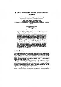
Figure 16: Fids time requirements

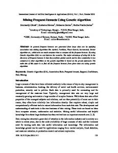
Figures 16 show time results itemsets. Every two batches (maxL = 2 in our experiments) the algorithm needs more time to process itemsets, this is in fact due to the merge operation of the tilted time windows which is done in our experiments every 2 batches. The jump in the algorithm is thus the result of extra computation cycles needed to merge the tilted time values for all the nodes in the Latticereg structure. We can notice that the time requirements of the algorithm as the stream progresses never excess the 30 seconds computation time limit for every batch. Figures 17 show memory needs for the processing of our itemsets. We can notice that the space requirement is bounded by 4.5M and thus can easily fit into main memory. Experiments show that the FIDS algorithm can handle itemsets in data streams without falling behind the stream as long as we choose correct batch duration values. 4.5e+06 Epsilon=0.1

Memoire utilisee (en Bytes)

4e+06

3.5e+06

3e+06

2.5e+06

2e+06 0

2

4

6

8

10 Batches

12

14

16

18

20

Figure 17: Fids memory requirements

15

6

Conclusion

In this paper we addressed the problem of mining itemsets in streaming data. Our main contributions are the following. First, by using prime numbers for representing items of the stream we improve the itemset inclusion checking and thus improve the overall process. Second, by using a new region-based structure we propose to efficiently find stored itemsets either for mining included itemsets or for pruning. Last, by storing only a minimal number of itemsets (i.e. the longest maximal itemsets) coupled with a tilted-time window, we can produce an approximate answer with an assurance that it will not bypass user-defined frequency and temporal thresholds. With Fids, users can, at any time, issue requests for frequent itemsets over an arbitrary time interval.

References [1] R. Agrawal, T. Imielinski, and A. Swami. Mining association rules between sets of items in large database. In Proc. of the Intl. Conf. on Management of Data (ACM SIGMOD 93), 1993. [2] Y. Chen, G. Dong, J. Han, B. Wah, and J. Wang. Multi-dimensional regression analysis of time-series data streams. In Proc. of VLDB’02 Conference, 2002. [3] Y. Chi, H. Wang, P.S. Yu, and R.R. Muntz. Moment: Maintaining closed frequent itemsets over a stream sliding window. In Proc. of ICDM’04 Conference, 2004. [4] P. Dokas, L. Ertoz, V. Kumar, A. Lazarevic, J. Srivastava, and P.-N. Tan. Data mining for network intrusion detection. In Proc. of the 2002 National Science Foundation Workshop on Data Mining, 2002. [5] G. Giannella, J. Han, J. Pei, X. Yan, and P. Yu. Mining frequent patterns in data streams at multiple time granularities. In Next Generation Data Mining, MIT Press, 2003. [6] J. Han, J. Pei, B. Mortazavi-asl, Q. Chen, U. Dayal, and M. Hsu. Freespan: Frequent pattern-projected sequential pattern mining. In Proc. of KDD’00 Conference, 2000.

16

[7] C. Jin, W. Qian, C. Sha, J.-X. Yu, and A. Zhou. Dynamically maintaining frequent items over a data stream. In Proc. of CIKM’04 Conference, 2003. [8] R.-M. Karp, S. Shenker, and C.-H. Papadimitriou. A simple algorithm for finding frequent elements in streams and bags. ACM Transactions on Database Systems, 28(1):51–55, 2003. [9] H.-F. Li, S.Y. Lee, and M.-K. Shan. An efficient algorithm for mining frequent itemsets over the entire history of data streams. In Proc. of the 1st Intl. Workshop on Knowledge Discovery in Data Streams, 2004. [10] G. Manku and R. Motwani. Approximate frequency counts over data streams. In Proc. of VLDB’02 Conference, 2002. [11] S.N. Sivanandam, D. Sumathi, T. Hamsapriya, and K. Babu. Parallel buddy prima - a hybrid parallel frequent itemset mining algorithm for very large databases. In www.acadjournal.com, Vol.13, 2004. [12] W.-G. Teng, M.-S. Chen, and P.S. Yu. A regression-based temporal patterns mining schema for data streams. In Proc. of VLDB’03 Conference, 2003.

17