A Fast Algorithm for Mining Utility-Frequent Itemsets - DTAI

A Fast Algorithm for Mining Utility-Frequent Itemsets Vid Podpeˇcan1 , Nada Lavraˇc1,2 , and Igor Kononenko3 1

Jozef Stefan Institute, Ljubljana, Slovenia University of Nova Gorica, Nova Gorica, Slovenia University of Ljubljana, Faculty of Computer and Information Science, Ljubljana, Slovenia 2

3

[email protected] [email protected] [email protected] Abstract. Utility-based data mining is a new research area interested in all types of utility factors in data mining processes and targeted at incorporating utility considerations in both predictive and descriptive data mining tasks. High utility itemset mining is a research area of utilitybased descriptive data mining, aimed at finding itemsets that contribute most to the total utility. A specialized form of high utility itemset mining is utility-frequent itemset mining, which – in addition to subjectively defined utility – also takes into account itemset frequencies. This paper presents a novel efficient algorithm FUFM (Fast Utility-Frequent Mining) which finds all utility-frequent itemsets within the given utility and support constraints threshold. It is faster and simpler than the original 2P-UF algorithm (2 Phase Utility-Frequent), as it is based on efficient methods for frequent itemset mining. Experimental evaluation on artificial datasets show that, in contrast with 2P-UF, our algorithm can also be applied to mine large databases.

1

Introduction

Utility-based data mining [10–12] is a broad topic that covers all aspects of economic utility in data mining. It encompasses predictive and descriptive methods for data mining, among the later especially detection of rare events of high utility (e.g. high utility patterns). This paper describes methods for itemset mining or more specifically, mining utility-frequent itemsets which is a special form of high utility itemset mining [13, 14]. Standard methods for association rule mining [1, 14] are based on support and confidence measures. The goal of the first phase of assoc. rule mining is to find all frequent itemsets and the goal of the second phase is to build rules based of frequent itemsets. We use support measure because we assume that the user is interested only in statistically important patterns. However, frequency of an itemset alone does not assure its interestingness because it does not contain information on its subjectively defined utility such

10

Vid Podpeˇcan, Nada Lavraˇc, Igor Kononenko

as profit in euros or some other variety of utility. Mining high utility itemsets thus upgrades the standard frequent itemset mining framework as it employs subjectively defined utility instead of statistics-based support measure. Userdefined utility is based on information not available in the transaction dataset. It often reflects user preference and can be represented by an external utility table or utility function. Utility table (or function) defines utilities of all items in a given database (we can also treat them as weights). Besides subjective external utility we also need transaction dependent internal utilities (e.g. quantities of items in transactions). Utility function we use to compute utility of an itemset takes into account both internal and external utility of all items in a itemset. The most usual form that is also used in this paper is defined as a sum of products of internal and external utilities of present items. The goal of high utility itemset mining is to find all itemsets that give utility greater or equal to the user specified threshold. The deficiency of this approach is that it does not consider the statistical aspect of itemsets. Utility-based measures should incorporate user-defined utility as well as raw statistical aspects of data [14]. Consequently, it is meaningful to define a specialized form of high utility itemsets, utility-frequent itemsets [15] which are a subset of high utility itemsets as well as frequent itemsets. Example 1 indicates differences between frequent, high utility and utility-frequent itemsets. Example 1. As an example let us analyze sales in a large retail store. We can find that itemset {bread, milk} is frequent, itemset {caviar, champagne} is of high utility and itemset {beer} is utility frequent. A smart manager should pay special attention to itemset {beer} as it is frequent and of high utility. On the other side, itemset {bread, milk} is frequent but not of high utility and itemset {caviar, champagne} gives high utility but is not frequent. First algorithm 2P-UF for mining utility-frequent itemsets was introduced together with formal definition of this novel area [15] of utility-based itemset mining. It is based on a quasi support, a special measure that solves the problem of nonexistence of anti-monotone property of joined support-utility measure. 2P-UF is proven to find all utility-frequent itemsets but it has some properties that render it impossible to use in practice on large databases. In this paper we present a new algorithm that treats utility-frequent itemsets as a special form of frequent itemsets which is in contrast with 2P-UF algorithm since it treats them as a special form of high utility itemsets. Our approach proves to be efficient because support measure has anti-monotone property and assures efficient mining approach. Moreover, it is possible to use existent, very efficient methods for mining frequent itemsets, that can significantly speed up the mining process. The remainder of this paper is organized as follows. In Section 2 we briefly survey work on frequent and high utility itemset mining as it forms a formal theoretical background for our algorithm. In Section 3 we describe our new algoritm and its advantages in comparison with 2P-UF algorithm. Section 4 describes and comments our implementation and results of experiments on synthetical

A Fast Algorithm for Mining Utility-Frequent Itemsets

11

databases. Finally, conclusions are drawn in Section 5 where we also indicate possible directions of future work.

2

Mining High Utility Itemsets

A frequent itemset is a set of items that appears at least in a pre-specified number of transactions. Formally, let I = {i1 , i2 , . . . , im } be a set of items and DB = {T1 , T2 , ..., Tn } a set of transactions where every transaction is also a set of items (i.e. itemset). Given a minimum support threshold minSup an itemset S is frequent iff: |{T |S ⊆ T, T ⊆ DB, S ⊆ I}| ≥ minSup . |DB| Frequent itemset mining is the first and the most time consuming step of mining association rules. During the search for frequent itemsets the anti-monotone property is used. Definition 1. Let D be the domain of a function f. f has the anti-monotone property when ∀ x, y ∈ D : x ≤ y ⇒ f (y) ≤ f (x). In the case of mining frequent itemsets the anti-monotone property assures that no superset of an infrequent itemset is frequent. Consequently, infrequent candidates can be discarded during the candidate generation phase. The first efficient frequent itemset mining algorithm APriori was developed by Agrawal et. al. [1], but later many faster methods were developed (FP-trees [5], ECLAT [16], Relim [2]). For the sake of simplicity, our implementation uses the APriori algorithm, however, any other more efficient algorithm could be used. 2.1

High Utility Itemsets

A high-utility itemset mining model was defined by Yao, Hamilton and Butz [13]. It is a generalization of the share-mining model [3, 4]. The goal of high utility itemset mining process is to find all itemsets that give utility greater or equal to the user specified threshold. The following is the set of definitions given in [13] which we shall illustrate on a small example. Definition 2. The external utility of an item ip is a numerical value yp defined by the user. It is transaction independent and reflects importance (usually profit) of the item. External utilities are stored in an utility table. For example, external utility of item B in Table 2 is 10. Definition 3. The internal utility of an item ip is a numerical value xp which is transaction dependent. In most cases it is defined as the quantity of an item in transaction. For example, internal utility of item E in transaction T5 is 2 (see Table 1).

12

Vid Podpeˇcan, Nada Lavraˇc, Igor Kononenko Table 1. Database with 10 transactions and 5 distinct items. TID 1 2 3 4 5 6 7 8 9 10

A 0 0 2 1 0 1 0 3 1 0

B 0 6 0 0 0 1 10 0 1 6

C 18 0 1 0 4 0 0 25 0 2

D 0 1 0 1 0 0 1 3 0 0

E 1 1 1 1 2 0 1 1 0 2

Table 2. External utilities of items from database in Table 1. item A B C D E profit (e) 3 10 1 6 5

Definition 4. Utility function f is a function of two variables: f (x, y) : (R+ , R+ ) → R+ . The most common form also used in this paper is the product of internal and external utility: xp ∗ yp . Definition 5. The utility of item ip in transaction T is the quantitative measure computed with utility function from Definition 4: u(ip , T ) = f (xp , yp ), ip ∈ T . For example: utility of item E in transaction T5 is 2 ∗ 5 = 10. DefinitionP 6. The utility of itemset S in transaction T is defined as u(S, T ) = u(ip , T ), S ⊆ T . For example: utility of itemset {B, E} in transip ∈S

action T2 is u({B, E} , T2 ) = u({B} , T2 ) + u({E} , T2 ) = 6 ∗ 10 + 1 ∗ 5 = 65. Definition 7. P The utility of item ip in itemset S is defined as u(ip , T ). For example, utility of item E in itemset {B, E} u(ip , S) = T ∈DB, S⊆T

is u(E, {B, E}) = u(E, T2 ) + u(E, T7 ) + u(E, T10 ) = 20. Definition P 8. The utility of itemset P S inPdatabase DB is defined as u(S, T ) = u(S) = f (xp , yp ). T ∈DB, S⊆T

T ∈DB, S⊆T ip ∈S

For example, utility of itemset {A, E} in database from Table 1 is u({A, E}) = u({A, E} , T3 ) + u({A, E} , T4 ) + u({A, E} , T8 ) = 33. Definition 9. The utility of transaction T is defined as u(T ) =

P

u(ip , T ).

ip ∈T

For example: utility of transaction T10 is u(T10 ) = u({B} , T10 ) + u({C} , T10 ) + u({E} , T10 ) = 72.


13

P

u(T ).

Definition 10. The utility of database DB is defined as u(DB) =

T ∈DB

For example, utility of database DB from Table 1 is u(DB) = u(T1 ) + . . . + u(T10 ) = 23 + . . . + 72 = 400. Definition 11. The utility share of itemset S in database DB is defined as u(S) . For example, utility share of itemset {A, D, E} in database from U (S) = u(DB) 46 Table 1 is U ({A, D, E}) = 400 = 0.115 = 11.5%. Finally, on the basis of definitions 2–11 we can formally define high utility itemset and the general problem of high utility itemset mining. Definition 12. Itemset S is of high utility iff U (S) ≥ minUtil where minUtil is user defined utility threshold in percents of the total utility of the database. Definition 13. High utility itemset mining is the problem of finding set H defined as H = {S|S ⊆ I, U (S) ≥ minUtil} where I is the set of items (attributes). Utility function from Definition 4 is neither monotone or anti-monotone which can be proven with a counter example based on database from Table 1: {A, E} ⊆ {A, D, E} , u({A, E}) ≤ u({A, D, E}) and {B} ⊆ {B, C} , u({B}) ≥ u({B, C}). Because of the nonexistence of anti-monotone property of utility function efficient high utility itemset mining algorithms [7, 8] employ critical function, a special function that estimates the utility of all possible supersets of a given itemset. It has the anti-monotone property which ensures the existence of a systematic non-exhaustive mining method. Critical function of itemset S is simply utility (see Definition 10) of database DBS (a subset of DB with only those transactions that contain S). It is used to reduce the number of candidates by discarding low quality itemsets (all their supersets are of low utility) during the candidate generation phase of the high utility itemset mining process. 2.2

Utility-Frequent Itemsets

Utility-frequent itemsets are a special form of high utiltity itemsets, therefore, all quoted definitions also apply. For a given utility threshold µ each itemset S is associated with a set of transactions defined as τS,µ = {T |S ⊆ T ∧ u(S, T ) ≥ µ ∧ T ∈ DB}. On the basis of this set of trans|τS,µ | . actions an extended support measure can be identified: support(S, µ) = |DB| Definition 14. Itemset S is utility-frequent if for a given utility threshold µ and support threshold s the extended support measure support(S, µ) is greater or equal to s. The measure of extended support is obviously not anti-mnotone as it is based on a non-monotone utility function (see Definition 4 and counter example). It is

14


possible to use critical function and algorithms for high utility itemset mining (i.e. DCG [7], ShFSM [8]), however, they are highly impractical and inefficient since the utility threshold is defined at transaction level instead of database level (see definition of the set τS,µ ) and thus much smaller. Because the utility threshold has direct influence on the number of candidates in DCG and ShFSM algorithm, they generate many high utility candidates (with respect to a given threshold). However, only a small fraction of them are also utility frequent. To tackle this problem, authors of the utility-frequent itemset mining model defined quasi support, the basis of their 2P-UF algorithm [15]. Definition 15. Quasi support is a special form of extended support defined ′ | |τS,µ ′ ′ where τS,µ is a set of transactions τS,µ = as quasiSupport(S, µ) = |DB| {T |u(S, T ) ≥ µ ∧ T ∈ DB}. We should remind the reader that it is not necessary for an itemset S to be a true subset of transaction T when computing its quasi support. It can be only partially contained as long as it gives desired minimum utility. Quasi support has the monotone property which ensures the existence of systematic non-exhaustive mining method. However, in comparison with the use of an antimonotone function the process runs in the opposite direction. Proof (monotonicity of the quasi support measure). Let X and Y be subsets of the set I (set of all items in a database) and let X ⊆ Y and let X be utility-frequent. ′ Obviously, for each transaction T ⊆ τX,µ holds u(Y, T ) ≥ u(X, T ) because X is ′ ′ a subset of Y. Thus, |τY,µ | ≥ |τX,µ |, quasiSupport(Y, µ) ≥ quasiSupport(X, µ) and Y is utility frequent. ⊓ ⊔ 2P-UF algoritm is based on the fact that every utility-frequent itemset is also quasi utility-frequent. Figure 1 briefly describes the 2P-UF algorithm. In the first phase of the algorithm all quasi frequent itemsets are collected and in the second phase all quasi utility-frequent but not utility-frequent are discarded. Function QU F − AP riori(·, ·, ·) starts with itemsets of length n − 1 (n is the number of items in DB). It computes intersection of each itemset with all other itemsets. Candidates of length n − 2 which do not have quasi utility-infrequent supersets (monotone property) and satisfy the given utility threshold are appened to the set of quasi utility-frequent itemsets and used in the next iteration to find all quasi utility-frequent itemsets of length n − 3. The process repeats until candidates of length 1 are generated and checked or the new set of candidates is empty and no shorter candidates can be produced. Further details of the 2P-UF algorithm and detailed description of the function QU F − AP riori(·, ·, ·) can be found in [15]. Mining of high utility and utility-frequent itemsets should be organized similar to mining of frequent itemsets. We start with conservative (high) thresholds and lower them as long as we are not contended with the number of itemsets found.


15

Algorithm 2P-UF Input: - database DB - constraints minUtil and minSup Output: - all utility-frequent itemsets /* Phase 1: find all quasi utility-frequent itemsets */ [1] CandidateSet = QUF-APriori(DB, minUtil, minSup) /* Phase 2: prune utility-infrequent itemsets */ [2] foreach c in CandidateSet: [3] foreach T in DB: [4] if c in T and u(c,T) >= minUtil: [5] c.count += 1 [6] return {c in CandidateSet | c.count >= minSup} Fig. 1. Pseudo code of the 2P-UF algorithm.

3


2P-UF utility-frequent itemset mining algorithm described in Section 2 is proven to find all utility-frequent itemsets. However, due to the monotone property of quasi support measure it has a few disadvantages which render it unusable for mining of large datasets. The first weak point is the reversed way of candidate generation. 2P-UF algorithm wastes time checking long itemsets that are highly unusual to be utility-frequent. For example, when mining a database with 1000 distict items (attributes) 2P-UF algorithm first generates and checks all itemsets of length 999, then itemsets of length 998 etc. Short itemsets which have fairly large probability to be utility-frequent, come at the very end. Candidate generation function is also slow and inefficient as it computes intersection of every pair of candidates in each iteration. Moreover, computation of quasi support measure is also inefficient because special data structures (hash trees) can not be used and we have to scan database once for every candidate. Finally, the two-phase form of the algorithm is space consuming since we have to store all quasi utility-frequent candidates from the first phase to filter them in the second phase. It is possible to avoid this waste of space by merging both phases and filter non utility-frequent candidates in every iteration of the algorithm. It is obvious that 2P-UF algorithm can not be used in practice where databases usually consist of millions of transactions and thousands of items. Our new algorithm [9] FUFM (Fast Utility-Frequent Mining) is based on the fact that utility-frequent itemsets are a special form of frequent itemsets. Moreover, the support measure is always greater or equal to the extended support measure. Proof is trivial because when computing extended support we count only those transaction containing given itemset S that also gives minimum utility on S,

16


but when computing ”ordinary” support we count all transactions containing S. The practical consequence of this statement is that frequent itemset mining algorithms can be used to mine utility-frequent itemsets. These algorithms are well studied and also very efficient. For this reason, our FUFM algorithm is very simple and fast because the main part is the ”external” frequent itemset mining algorithm. It is straightfoward to find utility-frequent itemsets among frequent itemsets because all that is needed is to build a hash tree. This data structure [1] is used to compute supersets (i.e. transactions) for all candidates and, with this information, utilities of all candidates. Figure 2 shows pseudo code of our FUFM algorithm.

Algorithm FUFM Input: - database DB - constraints minUtil and minSup Output: - all utility-frequent itemsets [1] L = 1 [2] find the set of candidates of length L with support >= minSup [3] compute exteded support for all candidates and output utilityfrequent itemsets [4] L += 1 [5] use the frequent itemset mining algorithm to obtain new set of frequent candidates of length L from the old set of frequent candidates [6] stop if the new set is empty otherwise go to [3] Fig. 2. Pseudo code of the FUFM algorithm.

Clearly, FUFM algorithm does not have disadvantages and inefficiencies of the 2P-UF algorithm as its generation phase (step 5 on Fig. 2) is based on frequent itemset mining methods. Filtering non-utility frequent candidates is also efficient because we only need to build a hash tree from candidates and push all transactions down the tree to compute subsets. Consequently, time and space complexity are both fully determined with the complexity of the frequent itemsets mining method used. Comparison of the number of candidates from consequent iterations of 2P-UF and FUFM algorithms is not trivial, but intuitively we can conclude that in first iterations of the 2P-UF algorithm there are lots of candidates since quasi support measure overestimates longer itemsets. In fact, 2P-UF algorithm is efficient only in case when utility threshold is very high and result is an empty set. In such case the mining process stops at the very first iterations. Because in our new algorithm utility threshold does not have influence on the candidate generation


17

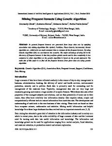
phase, FUFM performs worse in this special case as it has to inspect all frequent itemsets regardless of their utility. Let us compare the sets of generated candidates with 2P-UF and FUFM algorithm on a small database with 200 transactions. Utility threshold was set to 17.94 e (0.5% of the total utility of the database) and support threshold was fixed on 10%. Both algorithms found all 21 utility-frequent itemsets, FUFM in 8.5 seconds and 2P-UF in 1567.8 seconds. Number of remaining candidates (after prunning low support / non quasi utility-frequent candidates from all generated candidates) is represented with a graph on Fig. 3.

Fig. 3. Number of remaining candidates using 2P–UF and FUFM.

Let us point out again that 2P-UF algorithm generates utility-frequent itemsets in reverse order. Therefore, iteration i of the FUFM algorithm structurally equalls iteration 15 − i of the 2P-UF algorithm.

4

Experiments

Both algorithms were implemented in the Python programming language within the Orange [17] data mining framework. Our choice of interpreted programming language results in some severe constraints concerning the size of used databases. However, our implemetation is for testing purposes only and not for use in practice. All experiments were performed on a PC with AMD 3000+ processor, 512MB of main memory, version 2.5 of Python interpreter and Orange 0.99b (17th may 2007). We used IBM Quest synthetic data generator [1, 6]. It is highly advanced and considers typical properties of real transactional databases such as high frequencies of some itemsets, mean length of transactions, etc. This generator can produce only a binary form of transactional databases. Therefore, internal and external utilities were generated separately from the log-normal distribution in range [1, . . . , 10] (internal) and [1, . . . , 20] (external). Figure 4 shows rounded external utilities for 500 items.

18


Fig. 4. External utility distribution with 500 distinct items (log-normal distribution, shape parameter = 0.7).

Two databases with 50 000 and 100 000 transactions were used. They can be formalized in Quest notation as follows: T10.I4.D50000.N750, T10.I4.D100000.N1000 where T is the mean length of transaction, I is the mean length of potentially frequent itemsets, D is the number of transactions and N is the number of distinct items (attributes). 2P-UF algorithm is completely unusable on such large databases, therefore, we do not show its results as the execution was terminated manually due to extraordinary time complexity. We point the reader to the former example with 200 transactions to compare time complexity of both algorithms. Figure 5 shows the performance of the FUFM algorithm on database T10.I4.D50000.N750 with support threshold set to 0.5%.

Fig. 5. Number of utility-frequent itemsets and running time of the FUFM algorithm (database T10.I4.D50000.N750, minSup = 0.5%).

Red line connecting the columns shows execution time in seconds. As we already mentioned, the actual number of utility-frequent itemsets does not noticeably


19

influence the total running time of the algorithm. For that reason, the red line is straight and indicates the total running time of approx. 250 seconds. Table 3 shows the execution of FUFM algorithm on database T10.I4. D100000.N1000. With support threshold set to 0.1% and utility threshold to 147,95 e (0.001% of the total utility of the database) our algorithm finds all 121 utility-frequent itemsets in 1754 seconds. Number of generated candidates can be quite large (second row of the table), but after prunning all low support candidates the remaining number of high support candidates is perfectly acceptable (third row). For practical use the total time of 1754 seconds would be inacceptable, but it should be noted that implementation in C++ could be many times faster and appropriate for even larger databases. As a further improvement a faster frequent itemset mining method could be used instead of APriori. Table 3. Summary of execution of the FUFM algorithm on database T10.I4.D100000.N1000. minSup = 0.1%, minUtil = 147,95 e = 0.001% of total utility of DB. iteration generated candidates remaining candidates utility-frequent itemsets

5

1 2 3 4 5 6 870 320400 42011 5721 3292 1468 801 8783 7156 5563 3233 1441 5 3 12 25 26 22

7 500 494 17

8 131 131 10

9 23 23 1

10 2 2 0

11 0 0 0

Conclusions and Further Work

In this paper we introduced a novel, fast algorithm for mining all utility-frequent itemset. It is considerably faster than first algorithm 2P-UF and also much simpler to implement. Because it is based on efficient methods for mining frequent itemset it also performs well on real-sized databases. Our FUFM algorithm and 2P-UF algorithm were both implemented in Python and tested on a few synthetic databases generated with IBM Quest data generator. We plan to implement both algoritms in C++ together with a more advanced method for mining frequent itemsets. We also intend to test our algorithm on a real dataset from a retail store and analyze the results which could be used in practice.

References 1. Agrawal R., Imielinski T., Swami A.: Mining association rules between sets of items in large databases. Proceedings of the ACM SIGMOD Intl. Conf. on Management of Data, Washington, D.C., may 1993, pp. 207–216. 2. Borgelt C.: Keeping Things Simple: Finding Frequent Item Sets by Recursive Elimination. Workshop Open Source Data Mining Software, ACM Press, New York, pp. 66-70, 2005.

20


3. Carter C, Hamilton H. J., Cercone N.: Share based measures for itemsets. In Proc. First European Conf. on the Principles of Data Mining and Knowledge Discovery, pp. 14–24, 1997. 4. Hilderman R. J., Carter C. L., Hamilton H. J., Cercone N.: Mining market basket data using share measures and characterized itemsets. In Pacific-Asia Conference on Knowledge Discovery and Data Mining, pp. 159–170, 1998. 5. Han J., Pei J., Yin Y.: Mining frequent patterns without candidate generation. In Proceedings of the Int. Conf. on Management of Data, pp. 1–12, 2000. 6. IBM Almaden research center: Synthetic data generation code for associations and sequential patterns. Available at: http://www.almaden.ibm.com/cs/projects/iis/hdb/Projects/data mining /datasets/syndata.html/#assocSynData 7. Li Y. C., Yeh J. S., Chang, C. C.: Direct candidates generation: a novel algorithm for discovering complete share-frequent itemsets. In Proceedings of the 2nd Intl. Conf. on Fuzzy Systems and Knowledge Discovery, pp. 551–560, 2005. 8. Li Y. C., Yeh J. S., Chang, C. C.: Efficient algorithms for mining share-frequent itemsets. In Proceedings of the 11th World Congress of Intl. Fuzzy Systems Association, pp. 543–539, 2005. 9. Podpeˇcan V.: Utility-based Data Mining. BSc Thesis (in Slovene), University of Ljubljana, 2007. 10. ACM SIGKDD Workshop on utility-based data mining, 2005. Available at: http://storm.cis.fordham.edu/˜gweiss/ubdm-kdd05.html 11. 11.ACM SIGKDD Workshop on utility-based data mining, 2006. Available at: http://www.ic.uff.br/ bianca/ubdm-kdd06.html 12. Weiss G., Zadrozny B., Saar-Tsechansky M.: Utility-based data mining 2006 workshop report. SIGKDD Explorations, volume 8, issue 2. 13. Yao H., Hamilton H. J., Butz C. J.: A Foundational Approach to Mining Itemset Utilities from Databases. In The Fourth SIAM International Conference od Data Mining SDM, pp. 428–486, 2004. 14. Yao H., Hamilton H. J., Geng L.: A Unified framework for Utility based Measures for Mining Itemsets. Second International Workshop on Utility-Based Data Mining, Philadelphia, Pennsylvania, 2006. 15. Yeh J. S., Li, Y. C., Chang C. C.: A Two-Phase Algorithm for Utility-Frequent Mining. To appear in Lecture Notes in Computer Science, International Workshop on High Performance Data Mining and Applications, 2007. 16. Zaki M. J., Parthasarathy S., Ogihara M., Li W.: New Algorithms for Fast Discovery of Association rules. In Proceedings of the 3rd Intl. Conf. on Knowledge discovery and Data Mining, Newport Beach, California, pp. 283–286, 1997. 17. Zupan B., Demˇsar J., Leban G.: Orange: From Experimental Machine Learning to Interactive Data Mining. White Paper, (available at: www.ailab.si/orange), Faculty of Computer and Information Science, University of Ljubljana, 2004.