bounds to be given for all loops or recursive calls with ..... sor segments, s3 and s4. On the right hand ..... International Conference on Embedded and Real-Time.
Towards Adaptable Control Flow Segmentation for Measurement-Based Execution Time Analysis ∗ Michael Zolda
Sven B¨unte
Raimund Kirner
Real Time Systems Group Vienna University of Technology, Austria E-mail: {michaelz,sven,raimund}@vmars.tuwien.ac.at Abstract During the design of embedded real-time systems, engineers have to consider the temporal behavior of software running on a particular hardware platform. Measurement-based timing analysis is a technique that combines elements from static code analysis with execution time measurements on real physical hardware. Because performing exhaustive measurement is generally not tractable, some kind of abstraction must be used to deal with the combinatoric complexity of real software. We propose an adaptable measurement-based analysis approach that uses the novel flexible abstraction of a segment graph to model control flow at varying levels of detail. We also present preliminary experimental results produced by a prototype implementation.
1 Introduction In real-time systems the term correctness does not only refer to the functional behavior of calculations. Compliance with temporal requirements is an essential part in the design process. If transient violations of timing constraints are tolerated we speak of soft real-time systems. Think of a mobile phone for instance where short communication delays are acceptable. On the other hand, safetycritical hard real-time systems include at least one temporal requirement the violation of which would potentially lead to a catastrophe. An airbag not releasing in time or a non-reacting aircraft control unit for instance can lead to a fatal disaster. Consequently, there is an inherent demand for verification techniques that focus on the temporal behavior of real-time systems. Usually, a design is composed out of ∗ The
research leading to these results has received funding from the Austrian Science Fund (Fonds zur F¨orderung der wissenschaftlichen Forschung) within the research project Formal Timing Analysis Suite of Real-Time Systems (FORTASRT) under contract P19230-N13 and the research project ‘Sustaining Entire Code-Coverage on Code Optimization (SECCO) under contract P20944-N13.
tasks to handle complexity. A schedule ensures that functional as well as temporal dependencies are adhered to. Most of the common schedulability analysis techniques demand the knowledge of a safe upper bound of the worstcase execution time (WCET) for each single task. For hard real-time systems those deadlines are strict. However, soft real-time systems can tolerate violations to some degree. A comprehensive overview of WCET analysis techniques is given in [22]. In summary, determining the WCET is hard due to the inherent complexity and the partly complementary requirements to the analysis: • Safety is the property that the obtained WCET estimate may not underestimate the real WCET • Precision is an indicator of the deviation between the obtained WCET estimate and the real WCET • Performance of the WCET analysis denotes the amount of computational resources needed to perform the analysis • Accessibility of the WCET analysis covers aspects like available granularity of WCET results, the backannotation of WCET results to the source code, and the necessary effort to perform the WCET analysis on a new target hardware There are three categories in which the various WCET analysis techniques can be classified. In end-to-end black box testing the program is simply executed on a set of input data. The advantage is that the test environment is easy to set up. However, there is no way to state anything about precision or safety. In contrast, static analysis examines a software/hardware model of the system under investigation without executing the program. This approach allows for deriving safe and sufficiently precise execution time bounds, which makes it suitable for verifying safetycritical real-time systems [9]. Still, modeling and analyzing the system adequately takes much effort. It can even be impossible if the system behavior is too complex or partly unknown (e.g. the documentation provided by the
processor manufacturer may be incomplete w.r.t. temporal aspects). A third category encompasses measurementbased techniques, i.e. all approaches that combine execution time measurements and static program analysis. Measurement-based techniques is usually designed with the explicit goal to provide a trade-off between safety, precision on the one hand and performance, accessibility on the other hand. This article illustrates the overall architecture and segmentation technique for a flexible and easily accessible measurement-based approach that is supposed to give a WCET estimate where the precision depends on how much effort the developer is willing to invest. The overall goal is to make it applicable in several development stages of the system under investigation. We focus on soft realtime systems because we cannot in general avoid underestimation of the actual WCET. However, the method is still appropriate for hard real-time systems in an early stage of development when preliminary results are needed. The basic concepts of measurement-based timing analysis are discussed in Section 2, which is followed by a discussion of related work on measurement-based WCET analysis. Program segmentation, as described in Section 4, is the key strategy to provide an adjustable coverage metric for the systematic execution time measurements. The details of the algorithm for program segmentation are given in Section 5. In Section 6 we illustrate the setup of experiments on a prototype implementation of the Formal Timing Analysis Suite (F ORTAS)1 , which yields preliminary results regarding the applicability and consequences of adaptable program segmentation for WCET analysis.
2 Measurement-based Timing Analysis Measurement-based Execution Time Analysis (MBTA) is a hybrid WCET analysis technique, i.e., it combines static program analysis techniques and execution time measurements. As shown in Figure 1, measurement-based timing analysis typically consists of the following three phases: Analysis and Decomposition: For WCET analysis, the maximal end-to-end execution time of the software is of interest. In general, to obtain a perfectly accurate timing model, we would have to consider the execution time of all possible operation sequences that can be performed by the computer while executing the given computer program. Measuring all these sequences is in general intractable, as there are simply too many of them. Therefore, reducing the number of execution time measurements is crucial for MBTA. One way to do this is to decompose the program behavior into subsets and to ensure coverage on each subset. The control flow graph (CFG) is a common graphbased program representation in compiler construction, 1 http://www.fortastic.net
where nodes represent the operations of the software and where edges represent possible successive executions2. We have chosen to operate on the CFG as a good basis for MBTA, because the execution time depends largely on which specific instructions are executed. We use the technique of segmentation to decompose the CFG of ANSI C programs into smaller subgraphs. Depending on how we decompose the program into segments, we can adjust the trade-off between safety, precision on the one hand, and performance, accessibility on the on the other hand. Execution Time Measurement: Once the program is decomposed, the execution time is determined for each segment. We measure the execution time on the real hardware, allowing us to take hardware characteristics into account without modeling them in full detail. Timing Composition: Having performed systematic execution time measurements for each segment, the timing results from all segments have to be composed to obtain a WCET estimate. As said above, due to hardware features like pipelines, caches, or out-of-order executions, without additional precautions our MBTA approach will not provide sufficient state coverage to guarantee safe WCET bounds. Source Code
Analysis and Decomposition
Execution Time Measurement
Timing Composition
WCET Estimate
Figure 1: Measurement-based Timing Analysis. Our design choice of decomposing C programs based on their CFG and learning a hardware model closely related to the CFG has two major ramifications: Accessibility: the derived timing information can be related to the source code. At least at the granularity of our segmentations it is directly possible to assign timing values to source code regions representing a segment. It is also possible to relate the timing of individual paths within a segment back to the source 2 The traditional definition of a CFG does not allow for linear sequences of operations, i.e., the nodes must constitute so-called basic blocks. We relax this requirement and allow for general graphs, as the restriction the basic blocks is neither strictly necessary, nor particularly useful in our context.
code. However, due to compiler optimizations, this can sometimes lead to timing distributions that may not be obvious at the source code level. Here the user would have to investigate the generated code to fully understand the timing results. Overall, our approach provides the software developer with a convenient representation of the timing information. Furthermore, since we do not make use of a hardware model, any systems can be analyzed as long as the target platform offers the necessary means for measurement. Safety and Precision: the measurement-based timing analysis framework is generally used to provide WCET estimates of reasonable precision instead of safe WCET bounds. The WCET estimate can be potentially unsafe due to the following reasons: • Compiler optimizations can introduce new control flow paths, which may not be covered by our test data generation based on the program source code. This is a given fact with today’s compilers which can only be avoided by deactivating code optimizations. However, we are also working on a more intelligent approach where the goal is to let the compiler activate only those code optimizations that do not threaten the preservation of a selected code coverage [13]. The advantage of this approach is that it will be relatively easy to integrate it into existing compilers. • State coverage of hardware components is usually very hard to achieve by measurementbased timing analysis methods [14]. Thus, on hardware where the instruction timing depends on the current state of the processor, the WCET estimate provided by our method may miss the worst-case initial hardware state for an execution-time measurement. A workaround to this problem would be the explicit enforcement of a predictable state at wellknown program points [20]. Measurementbased WCET analysis can potentially outperform static WCET analysis in precision. However, due to the statistical operation of measurement-based WCET analysis, this cannot be guaranteed. The discussions so far leads to the following main requirement for our measurement-based WCET analysis: The degree of precision and safety of the analysis has to be adaptable to the resources (e.g. analysis time) the developer is willing to invest. All involved means have to be conveniently accessible and capable of being integrated smoothly into a design process at multiple stages.
One way to achieve this goal is to make use of techniques where the level of abstraction is adaptable. We use program segmentation for splitting the CFG into overlapping subgraphs called segments. Each segment is small enough to be measured exhaustively w.r.t. path coverage (also referred to as predicate coverage [16]). The implicit premise of path coverage is that there is only a finite number of paths that need to be considered. Practically, this amounts to ruling out infinite loops and infinite recursion, which is a reasonable assumption for the kind software components we consider. Concretely we assume each task to be analyzed to be a so-called transformative system, i.e., a subsystem that takes its input data and transforms them into output data [2]. Following common practice, we assume the availability of iteration bounds for all cycles in the CFG. In many cases, such bounds can be derived automatically via static analysis techniques [7, 6]. Otherwise they must be provided by a human expert. The input data for the measurements is produced by FS HELL [10, 11], a database engine dispatching queries about a C program to program analysis tools. The version at hand utilizes the bounded model checker CBMC [5], which supports full ANSI-C, including function-pointers, bit-operations, and floating-point arithmetic. As a result, FS HELL is able to cope with full ANSI-C, but—due to the nature of bounded model checking—requires loop bounds to be given for all loops or recursive calls with non-constant bounds. For deriving a global WCET estimate we use the Implicit Path Enumeration Technique (IPET) [17, 15], for which the segment graph forms the input, i.e., the linear equations model the flow between segments and the cost for a segment is the worst case observed execution time thereof. As we will show, the segment size inherently affects analysis complexity and precision and must therefore be adaptable to satisfy our main requirement of having the precision and safety adaptable. Moreover, we will see that segments can be formed out of any graph-like structure such that hardware effects can potentially be incorporated. This enables our measurement-based WCET analysis to increase the level of precision and safety.
3 Related Work A means for control flow segmentation is discussed in [12] where the program is decomposed into a hierarchical tree of Regions. Each region has a single entry and a single exit (SESE) like our segments. We do not make use of any hierarchical structure, though. Furthermore, the presented algorithm to form the regions does not specifically target the reduction of possible control flow paths. Bernat et al. [3] and Ernst et al. [8] use program segmentation explicitly to target WCET analysis. Because they do not address the problem of systematic generation of input data and the implicit goal of reducing control flow
paths, both the structures and the segmentation algorithms differ from ours. Our work is largely motivated by Wenzel et al. [21]. The idea of CFG partitioning to reduce the amount of local paths for exhaustive measurements and the successive compositions of timing information for WCET calculation is first discussed in their work. We extend the segmentation to deal with loops and unstructured code. Furthermore, our approach is more flexible in the sense that we extend the degree of freedom for decomposition. The idea for an adaptable abstraction by using segments is discussed in [1]. However, while we decompose the CFG, their segmentation splits the IPET equation system for reducing complexity.
4 Segmentation To obtain a perfectly accurate timing model, we generally have to consider the execution time of all possible operation sequences that can be performed by the computer while executing the given computer program. In compiler construction, the traditional program representation that makes all statically possible operation sequences explicit is the control flow graph (CFG), a graph where nodes represent the operations of the software, and where edges represent possible successive execution. There are richer graph-like system representations for the set of possible operation sequences, like, e.g., the kripke structures used in formal methods, which can encode detailed information on the system state (the CFG merely distinguishes different code locations). Also, it is possible to enrich a CFG with additional state information, e.g., by using preconditions. In this paper we will only consider plain CFGs, but it should be noted that the concepts presented here can be adapted to other graph-like representations on different levels of abstraction. A CFG does not include information about the dynamics of the software. It therefore overapproximates the (dynamically) feasible operation sequences, a subset of all statically possible operation sequences. More precisely, each path through the CFG (from a distinguished start node to a distinguished end node) represents a (statically) possible operation sequence. By considering all these paths, we can conclude about the timing behavior of the complete program, from the timing behavior of the individual paths. For example, if we know the Worst Case Execution Time (WCET) of each path, we could, in principle, derive the WCET of the complete program. Consider the C source code in Listing 1. We can see that the false branch of the second conditional statement cannot be taken, if the false branch of the first conditional statement has been taken before. As a consequence, only three of the four statically possible paths through the corresponding CFG (Figure 2) are feasible. The infeasible path e7 , e6 , e3 , e2 does not contribute to the timing behavior of the program, because it can never
Figure 2: Maxseg segment graph induced by the program in Listing 1, an equivalent of the programs CFG. There are four statically possible paths. Assuming that edges 5 and 2 correspond to a successful test of the conditions x != 0 and x % 2 == 0, respectively, the path e7 , e6 , e3 , e2 is dynamically infeasible. i f ( x != 0) flags = 1; else flags = 0; i f ( x % 2 == 0 ) flags = flags | 2; else flags = flags | 4;
Listing 1: Source code of a program with two consecutive tests, where the second test can only fail after the first test has succeeded.
be executed. It should therefore be excluded from timing analysis. The CFG alone cannot represent this information. What we would like to have is a representation that is expressive enough to represent individual paths. However, considering the prohibitively large number of paths in most real software, the representation must also be capable of representing collections of paths concisely. Lastly, our representation should be similar to a CFG, so that timing analysis methods like IPET, which operate on a CFG, can be used with minimal adaption. Definition 1 (Segment Graph) A segment graph Σ of a CFG G is a tuple hG, S, I, nodes, edges, entry, exiti, where G = hN, E, init, f inali is a CFG with nodes N , edges E ⊆ N × N , an unique initial node init ∈ N , and an unique final node f inal ∈ N . Moreover, S is a set of segment names, I ⊆ S × S is a set of inter edges (edges between segments), nodes : S → P(N ) is a function designating the nodes in each segment, edges : S → P(E) is a function designating the edges in each segment, entry : S → N is function designating
the entry node of each segment, and exit : S → N is a function designating the exit node of each segment. For any inter edge hs, ti, we require that hexit(s), entry(t)i ∈ E. An intra edge in a segment s is an edge hv, wi with hv, wi ∈ edges(s). Each node and each intra edge must be in at least one segment, i.e., [ [ nodes(s) = N and edges(s) = E. s∈S
s∈S
Furthermore, entry and exit nodes must be in their corresponding segments, i.e., {entry(s), exit(s)} ⊆ nodes(s). Moreover, the source and target nodes of all intra edges must also be in the corresponding segment, i.e., hv, wi ∈ edges(s) ⇒ v ∈ nodes(s) ∧ w ∈ nodes(s). An initial segment is a segment s with init ∈ nodes(s). Likewise, a final segment is a segment s with f inal ∈ nodes(s). A segment path π(s) through a segment s is a sequence π(s) = hv1 , v2 ihv2 , v3 i . . . hvn−2 , vn−1 ihvn−1 , vn i of intra edges hvi , vi+1 i that are all in the segment s, i.e., hvi , vi+1 i ∈ edges(s), for some s ∈ S. Moreover, the path must start in the segment’s entry node and end in the segment’s exit node, i.e., v1 = entry(s) and vn = exit(s). Figure 3 visualizes a segmentation of the CFG from Figure 2 with three segments. We can seen that segments s1 and s3 are initial segments, because they contain the CFG’s initial node, whereas segments s2 and s3 are final segments, because they contain the CFG’s final node. Entry and exit of each segment indicated by dashed or dotted borders, respectively. We can see that nodes and intra edges can be shared between segments. Although not shown in this figure, it is also possible that an inter edge can at the same time be an intra edge for some segments. Semantically, a segment graph of a CFG G is a description of a subset of the paths in G. A segment graph can therefore be seen as a restriction of a CFG to a certain set of paths. Definition 2 (Paths in a Segment Graph) Let Σ be a segment graph hG, S, nodes, edges, entry, exiti. The set of paths in Σ is the set of all CFG paths π = π1 (s1 )e1 π2 (s2 )e2 . . . en−1 πn (sn ), where the πi si are segment paths that constitute dynamically feasible subpaths in G, and where ei = hexit(si ), entry(si+1 )i, i.e., the segment paths are connected via inter edges.
It can be shown that the set of paths in a segment graph of a CFG G is a subset of the paths in G. There are two interesting special cases of segment graphs: minseg: The minseg segment graph is the segment graph where each node is contained in its own segment, and where no segment contains any edge, i.e., nodes(sv ) = {v}, for any v ∈ N , edges(sv ) = ∅, entry(sv ) = v, and exit(sv ) = v. The paths in a minseg segment graph of a CFG G are the statically possible paths described by G. maxseg: There is a single segment s, which contains all nodes and edges of the CFG, i.e., nodes(s) = N , edges(s) = E, entry(s) = init, and exit(s) = f inal. The paths in a maxseg segment graph of a CFG G are the dynamically feasible paths of G. Applying the semantic definitions on the segment graph visualized in Figure 3, we obtain the following segment paths: s1 :{e5 } s2 :{e1 e0 , e3 e2 } s3 :{e7 e6 e1 e0 , e7 e6 e3 e2 }. Because the path e7 e6 e3 e2 is a dynamically infeasible path, the set of paths in the segment graph is {e5 e1 e0 , e5 e3 e2 , e7 e6 e1 e0 }.
Figure 3: A segment graph that was obtain from the one in Figure 2 by splitting at edge e4 . In this example the segment split into three smaller segments. Segment s1 now holds all paths that went from the original entry node of the prevision segment to the source node of the split edge, without passing the split edge itself. Segment s2 contains all paths that went from the target node of the split edge to the exit node, without passing the split edge itself. Segment s3 contains all paths that went from the entry node to the exit node, without passing the split edge. Edge e4 has become an inter edge. The segment graph framework as presented here does not include any special construct for handling function
calls. However, function calls are easily supported via inlining the body of called functions at their respective call sites. This approach allows for unrestricted segments across calling borders. On the other hand, function calls that have not been inlined are handled transparently, as atomic operations. This black-box view can be particularly useful in the case of closed-source third-party code.
5 Segmentation Algorithm For a given CFG, many different segment graphs are possible, so which one should we choose for our purpose of measurement-based timing analysis? The two corner cases are minseg and maxseg. The minseg segment graph is only interesting for comparison purposes, as it describes the same set of paths as the plain CFG. On the other hand, performing an analysis on a maxseg segment graph would mean that all statically possible paths have to be checked for feasibility and, in case they are found feasible, be subject to measuring and analysis. In this paper, we consider a segmentation algorithm that is based on the following idea: in order to exclude from the analysis as many infeasible paths as possible, we would like to have segments that are as large as possible in terms of the total number of segment paths. However, the total number of segment paths must not become too large, because we can only check, measure, and analyze a limited number of paths. Our algorithm starts out with a maxseg segment graph and iteratively splits segments into smaller segments until the number of segment paths3 is small enough in each segment. Because we have ruled out infinite loops, the number of paths in a segment is always finite and can be calculated as exact or approximate solution of a combinatorial problem that incorporates the given iteration bounds. Segments are always split at some intra edge and are thereby reduced to up to four smaller segments–details follow below. The new segments are put into a priority queue that is ordered by the number of segment paths. Multiple copies of the same segment are merged into a single segment, as soon as they occur. The algorithm keeps on splitting the largest segment (unless it is already small enough) until the queue is empty. As split edge, the algorithm chooses an edge with a maximal edge betweenness centrality measure. Edge betweenness is a centrality measure for graphs that indicates the relative importance of an edge as a passageway for shortest paths. It is defined as Σv,w∈N
σv,w (e) , σv,w
(1)
where σv,w designates the number of different shortest paths4 from node v to node w, and where σv,w (e) desig3 An
alternative measure is the total number of paths over all seg-
ments. 4 I.e., shortest statically possible CFG paths, in our case.
nates the number of shortest paths from node v to node w that pass through edge e. The rationale for choosing an edge with maximal edge betweenness for splitting is that cutting such an edge will produce new segments of considerably smaller size than the original segment, i.e., the algorithm will converge to a solution quickly. Moreover, the solution will feature relatively few, but large segments, which can be advantageous during further analysis, e.g., to keep the constraint system in an IPET analysis small. Edge betweenness can be computed very efficiently. Brandes [4] presents a method for computing betweenness and related shortest-path based centrality measures. The algorithm has an asymptotic worst-case time complexity of O(n·m), and an asymptotic worst-case space complexity of O(n + m), where n and m are the number of nodes and edges in the graph, respectively. Our current implementation of segmentation makes use of the BGL [18, 19] implementation of Brandes’ algorithm. Algorithm 1 illustrates our implementation. Algorithm 1 Pseudo code of the maximum betweenness segmentation algorithm. 1: procedure SEGMENTATE MAXBET (cf g, limit) 2: g ← maxseg segment graph of cf g 3: s ← the segment of g 4: insert s into priority queue q 5: while q is not empty do 6: pop segmentation s from q 7: if number of paths in s > limit then 8: e ← intra edge of s w/max. betweenness 9: new segments ← split s at edge e 10: replace s with new segments in g 11: insert new segments into q 12: merge equivalent segments in q 13: end if 14: end while 15: return g 16: end procedure
Splitting Splitting a segment s at an intra edge (v, w) means removing (v, w) from s and turning it into one or more inter edges e1 , . . . , en that connect the segments in the segment graph in such a way that, semantically, no dynamically feasible path is lost. When the split edge is removed, the previous segment breaks into up to four new segments: tosplit segment: A segment capturing all paths in the previous segment s from node entry(s) to node v that do not pass through edge (v, w). fromsplit segment: A segment capturing all paths in the previous segment s from node w to node exit(s) that do not pass through edge (v, w).
bypass segment: A segment capturing all paths in the previous segment s from node entry(s) to node exit(s) that do not pass through edge (v, w). loop segment: A segment capturing all paths in the previous segment s from node w to node v that do not pass through edge (v, w). Figure 4 shows how these segments are connected by inter edges. Figures 5 and 6 show a concrete example of splitting at a back edge. Figure 6: A segment graph that was obtained from the one in Figure 5 by splitting at the back edge e8 . Because the previous segment contained a loop, loop segment s3 was produced. This segment can be reached directly from the tosplit segment, and directly reaches the fromsplit segment, as well as itself, via a self loop.
Figure 4: Connection scheme of new segments after splitting. The left hand side shows segment s together with two predecessor segments, s1 and s2 , and two successor segments, s3 and s4 . On the right hand side s has been replaced by the new segments tosplit, f romsplit, bypass, and loop. These segments have been connected among each other as well as to their environment.
maximum betweenness segmentation algorithm, as presented above, can produce a large number of identical segments. Mostly, this happens when overlapping segments with a common entry or exit node are found to have their maximum betweenness in a shared edge. Our implementation of the maximum betweenness segmentation algorithm can optionally be configured to merge identical segments after each splitting step, which can reduce the size of the intermediate and final segment graphs significantly. During our experimental evaluation, our optimized segmentation algorithm was seen to work fine in practice. For a formal worst case complexity analysis of the algorithm, one would have to consider the combination of two diametrically opposed tendencies. On the one hand, each splitting step will replace a segment with up to four smaller segments. Even though many of these segments are immediately collapsed by the subsequent merging step, this can lead to exponential space complexity in the number of splitting steps. On the other hand, however, the bypass segment yielded by splitting is linearly smaller (in terms of paths) than the original segment. Moreover, the size of the to split, from split, and loop segments yielded by splitting at the edge with maximum betweenness is typically a fractional power of the size of the original segment. We have not performed a formal analysis of the overall space and time complexity of our algorithm.
6 Experiments Figure 5: A maxseg segment graph of a CFG that contains a loop.
Complexity Considerations In the course of repeated splitting, it may happen that some of the produced segments are very similar. In particular, our experimental evaluation showed that the plain
To highlight the adaptable character of the segmentation techniques we will compare two segmentations of the same input program. They represent two extreme cases where the first includes segments as large as possible (at most 100 paths per segment, i.e. test case generation is barely feasible for the number of contained paths) and the second one forms a single segment for each CFG node (i.e. one path per segment), respectively. This way we illustrate the dependency between analysis complexity and
Host A Segmentor
Measurement
Database
Repository Core
FShell
Controler IPET
C Modeler
Host B Core
Figure 7: The F ORTAS architecture. the WCET estimate’s precision. We utilize the F ORTAS framework to perform our experiments by which means we have access to all basic functions we need. Figure 7 illustrates the F ORTAS architecture that combines a collection of modules/plugins. The core manages the communication between these plug-ins by distributing XML-RPC protocol messages. It potentially allows for running plug-ins on different hosts for instance to parallelize the measurement and the test case generation processes. The presented algorithm is implemented in the segmentor. It gets the CFG from C modeler, an extension of LLVM and the Clang frontend. The derived segment graphs are added to the repository plug-in which provides a consistent and persistent way to access both intermediate and final analysis results. For each segment, we automatically derive a query for FS HELL [10, 11] which in turn generates a test data set yielding path coverage for the according segment. A query to FS HELL is formed by a sequence of program locations such that the generated input data result in an execution sequence including those locations. The input language also includes negations to exclude code locations for a test case and commands to target coverage metrics. By these means, each path in a segment can be expressed by the sequence of its CFG nodes. Query generation is therefore straightforward and convenient. Once all test data are generated, the consecutive measurement process takes the input data set and performs execution time measurements on the target platform. In a next step the longest observed execution time for each segment is filtered out from all measurements. The IPET plug-in assembles those values and the segment graph to apply the implicit path enumeration technique, yielding a global WCET estimate. The so far unmentioned controller implements the demonstrated work flow as well as means of logging, monitoring and verification. All plugins and the core run on a 2.66 GHz Intel Core2 Quad host with 8 GB of RAM. Target Platform and Measurement We perform measurements on an Infineon TriCore TC1796 microcontroller. It includes an instruction cache
and a processor pipeline which leads to potential underestimations of the global WCET since we do not incorporate execution histories at segment entries on the one hand. We also cannot capture all data-dependent execution time jitter on the other hand, as the CFG is a too coarse abstraction. However, for less complex hardware, e.g. the HCS12 microcontroller, the introduced timing analysis produces a safe WCET bound. We have chosen the TriCore for our measurements, because we plan to tackle the shortcomings of the approach w.r.t. complex hardware in the near future. Furthermore, the TC1796 includes On-Chip Debug Support (OCDS) level 2, providing means for cycleaccurate execution tracing. We utilize the Lauterbach LA-7690 Powertrace device to document both timing and flow of control, rendering code instrumentation obsolete: not only measurements have a higher resolution, also the source code can remain unchanged. A measurement starts with test data injection right before the call of the main function where all relevant registers (e.g. function arguments) and global variables are set. Note, that the hardware state (cache, pipeline, etc.) is unknown at this point. However, due to a previous initialization script this state is identical for every measurement. The measured execution (or trace) then includes not only the execution of main but also of all its children in the function call graph. In a postprocessing phase the resulting trace is related to the source code, its CFG and segments by the Measurement plug-in using debug information from the binary. OCDS Level 2 provides traces of temporally high resolution, i.e. every executed machine instruction gets a time stamp. Consequently, the duration of a measured segment path can be derived precisely as the machine instructions can be related to all CFG nodes in the corresponding segment. If measurements are too coarse, not every CFG node of a path through a segment will get a time stamp. This happens for instance when software instrumentation is used to raise hardware signals at certain program points to externally assign timestamps. In this case we choose the splitting edges during segmentation such that they are near to CFG nodes that can be mapped to a time stamp. Consequently, the level of freedom in choosing segment borders is an important feature for guaranteeing portability of our approach. One problem that comes along with OCDS is that the trace buffer might overflow if too many control flow changing instructions follow in succession. A lack of timing information in the trace influences measurement precision if it occurs at segment borders in which case the first/last available time stamp after/before the gap is taken as a reference for calculating the duration of a segment path. Although this potentially introduces a source of pessimism, we did not observe any trace gaps so far for any benchmark. Benchmark The input program on which we carried out the analysis is an engine control unit implemented in ANSI C. The reason for choosing the benchmark is manifold: (a) it rep-
resents a practical application from the automotive industry (provided by Magna Steyer Fahrzeugtechnik), (b) the code is generated by Matlab/Simulink and demonstrates that the analysis can potentially be integrated into a modern design process, (c) with 2952 source code lines and a size of 201430 bytes, it is considerably large and (d) it involves a complex control flow structure (1632 CFG nodes, 2164 transitions) with more than 1045 statically possible paths. The target function has one subfunction which is called at most three times per execution. The benchmark includes 230 integer variables that potentially affect control flow. Unfortunately, we cannot make the benchmark publicly available due to a non-disclosure agreement. 1 2 3 4 5 6 7 8 9 10 11 12 13 14
Paths per Segment Number of segments Sum of statically possible segment paths Sum of feasible segment paths Analyzed and/or measured paths Segmentation time [s] Test case generation time [s] Measurement [s] IPET time [s] Overall analysis time [s] Analysis time / path [s] WCET estimate [µs] WCOET [µs] Pessimism [%]
1 1287 1287 1201 387 166 6025 4447 1423 12061 20 20789 728 2756
≤ 100 73 2139 1403 2139 81 177464 10706 0.005 188251 83 1975 728 171
Table 1: Summarized results.
Preliminary Results The relation between maximal number of paths per segment, analysis complexity and precision is illustrated in Table 1. We see the results for two segmentations with a maximum of 1 and 100 paths per segment, respectively. The most important effects of these parameters, i.e. analysis complexity and precision are emphasized in rows 10 and 14: the more time is spent the less pessimistic the WCET estimate gets. Here, pessimism is defined as the difference between WCET estimate and the worst-case observed execution time (WCOET), divided by the WCET estimate. There were no manual efforts to maximize the WCOET, i.e. the WCOET is the execution time of maximal observed length. Note, that this metric is only an approximation for this target hardware. However, comparing WCOET and WCET estimate is the best metric available. The overall analysis time comprises applying the segmentation algorithm (6), test case generation via FS HELL (7), measuring the feasible segment paths (8) and timing composition via IPET (9) to get a WCET estimate. Test case generation uses up most of the analysis time: it has to generate input data or prove infeasibility for each statically possible segment path in each segment. The difference in analysis time per path is due to an optimization technique. In the experiment with one path per segment, we instructed FS HELL to generate input
data yielding basic block coverage for the whole program which implies path coverage for each segment in this special case. This also causes the reduced set of 387 out of 1287 paths that had to be analyzed and measured. In contrast, using a path bound of 100, all 2139 statically feasible paths have to be analyzed individually. A critical point that we observe is the too pessimistic estimate for a path bound of 1. Our major concern is now to find better segmentation parameters and to improve the overall performance such that useful results can be derived over night. Potential for Optimization So far, measurement and test case generation are processed sequentially although they can be pipelined. Table 1 shows that measurements are too time consuming. This is due to a bottleneck in our prototypical measurements device and will be improved in the future. All measurements are performed end-to-end such that a program execution causes the control flow to pass multiple segments sequentially. However, we do not test whether there is already a measurement in the repository for the segment path that we want to cover. We expect a drastic performance enhancement for this optimization technique. Another option which is not accounted for so far is to initially apply heuristic test case generation prior to model checking. This technique proved to boost performance considerably in [21].
7 Conclusion and Outlook In this paper we presented a measurement-based timing analysis approach that incorporates an abstraction technique to express a real-time system’s temporal behavior a varying levels of detail. This enables the analysis to be adaptable in terms of complexity, precision and safety. We have introduced the segment graph as a novel, flexible control flow abstraction that can be used to exclude dynamically infeasible paths from further analysis. As a basic operation on a segment graph, we have presented the splitting of individual segments at a given intra edge. This operation forms the foundation of the maximum betweenness segmentation algorithm, which tries to heuristically find a good segmentation. Although we have only considered CFG-like program representations in this paper, the concept of a segmentation graph is not restricted to this representation. Segmentation graphs can be constructed over other graph-based representations, like, e.g., kripke structures. Lastly, we have presented preliminary results of experiments that were performed using a prototype implementation of our approach. Immediate next steps are the further improvement of our prototype implementation which is still in an early stage of development, and performing further experiments. Our more ambitious plans include the develop-
ment of an adaptive analysis approach that employs an incremental refinement strategy to improve the analysis results. Acknowledgments. We are grateful to Michael Tautschnig and Andreas Holzer for providing FS HELL and the C Modeler. We also thank them for discussions on the topic of this paper.
References [1] C. Ballabriga and H. Cass´e. Improving the WCET Computation Time by IPET Using Control Flow Graph Partitioning. In R. Kirner, editor, 8th Intl. Workshop on WorstCase Execution Time (WCET) Analysis, Dagstuhl, Germany, 2008. Schloss Dagstuhl - Leibniz-Zentrum fuer Informatik, Germany. [2] K. Berkenk¨otter and R. Kirner. Model-based Testing of Reactive Systems, volume 3472 of Lecture Notes in Computer Science, chapter Real-Time and Hybrid Systems Testing, pages 355–387. Springer, July 2005. [3] G. Bernat, A. Colin, and S. M. Petters. WCET Analysis of Probabilistic Hard Real-Time Systems. In RTSS ’02: Proceedings of the 23rd IEEE Real-Time Systems Symposium, page 279, Washington, DC, USA, 2002. IEEE Computer Society. [4] U. Brandes. A Faster Algorithm for Betweenness Centrality. Journal of Mathematical Sociology, 25:163–177, 2001. [5] E. Clarke, D. Kroening, and F. Lerda. A Tool for Checking ANSI-C Programs . In K. Jensen and A. Podelski, editors, Tools and Algorithms for the Construction and Analysis of Systems (TACAS 2004), volume 2988 of Lecture Notes in Computer Science, pages 168–176. Springer, 2004. [6] M. de Michiel, A. Bonenfant, H. Cass, and P. Sainrat. Static Loop Bound Analysis of C Programs Based on Flow Analysis and Abstract Interpretation. In IEEE International Conference on Embedded and Real-Time Computing Systems and Applications (RTCSA), Kaohsiung, Taiwan, 25/08/2008-27/08/2008, pages 161–168, http://www.computer.org, aot 2008. IEEE Computer Society. [7] A. Ermedahl, C. Sandberg, J. Gustafsson, S. Bygde, and B. Lisper. Loop Bound Analysis based on a Combination of Program Slicing, Abstract Interpretation, and Invariant Analysis. In C. Rochange, editor, 7th Intl. Workshop on Worst-Case Execution Time (WCET) Analysis, Dagstuhl, Germany, 2007. Internationales Begegnungsund Forschungszentrum f”ur Informatik (IBFI), Schloss Dagstuhl, Germany. [8] R. Ernst and W. Ye. Embedded Program Timing Analysis Based on Path Clustering and Architecture Classification. In ICCAD ’97: Proceedings of the 1997 IEEE/ACM international conference on Computer-aided design, pages 598–604, Washington, DC, USA, 1997. IEEE Computer Society. [9] R. Heckmann and C. Ferdinand. Worst-case execution time prediction by static program analysis. White Paper, AbsInt Angewandte Informatik GmbH, 22nd May 2009.
[10] A. Holzer, C. Schallhart, M. Tautschnig, and H. Veith. FShell: Systematic Test Case Generation for Dynamic Analysis and Measurement. In Proceedings of the 20th International Conference on Computer Aided Verification (CAV 2008), volume 5123 of Lecture Notes in Computer Science, pages 209–213, Princeton, NJ, USA, July 2008. Springer. [11] A. Holzer, C. Schallhart, M. Tautschnig, and H. Veith. Query-Driven Program Testing. In N. D. Jones and M. M¨uller-Olm, editors, Proceedings of the Tenth International Conference on Verification, Model Checking, and Abstract Interpretation (VMCAI 2009), volume 5403 of Lecture Notes in Computer Science, pages 151–166, Savannah, GA, USA, January 2009. Springer. [12] R. Johnson, D. Pearson, and K. Pingali. The Program Structure Tree: Computing Control Regions in Linear Time. SIGPLAN Not., 29(6):171–185, 1994. [13] R. Kirner. Towards preserving model coverage and structural code coverage. EURASIP Journal on Embedded Systems, 2009, 2009. doi:10.1155/2009/127945. [14] R. Kirner and P. Puschner. Obstacles in worst-cases execution time analysis. In Proc. 11th IEEE International Symposium on Object-oriented Real-time distributed Computing, pages 333–339, Orlando, Florida, May 2008. [15] Y.-T. S. Li and S. Malik. Performance Analysis of Embedded Software Using Implicit Path Enumeration. SIGPLAN Not., 30(11):88–98, 1995. [16] S. C. Ntafos. A Comparison of Some Structural Testing Strategies. IEEE Trans. Softw. Eng., 14(6):868–874, 1988. [17] P. P. Puschner and A. V. Schedl. Computing Maximum Task Execution Times — A Graph-BasedApproach. RealTime Syst., 13(1):67–91, 1997. [18] J. G. Siek, L.-Q. Lee, and A. Lumsdaine. The Boost Graph Library: User Guide and Reference Manual (C++ InDepth Series). Addison-Wesley Professional, December 2001. [19] J. G. Siek, L.-Q. Lee, and A. Lumsdaine. The Boost Graph Library. http://www.boost.org/doc/libs/1_ 39_0/libs/graph/, Juli 2009. [20] I. Wenzel. Measurement-Based Timing Analysis of Superscalar Processors. PhD thesis, Technische Universit¨at Wien, Institut f¨ur Technische Informatik, Treitlstr. 3/3/182-1, 1040 Vienna, Austria, 2006. [21] I. Wenzel, B. Rieder, R. Kirner, and P. Puschner. Automatic Timing Model Generation by CFG Partitioning and Model Checking. In Proc. Conference on Design, Automation, and Test in Europe, Mar. 2005. [22] R. Wilhelm, J. Engblom, A. Ermedahl, N. Holsti, S. Thesing, D. Whalley, G. Bernat, C. Ferdinand, R. Heckmann, T. Mitra, F. Mueller, I. Puaut, P. Puschner, J. Staschulat, and P. Stenstr¨om. The Worst-Case Execution-Time Problem — Overview of Methods and Survey of Tools. ACM Trans. Embed. Comput. Syst., 7(3):1–53, 2008.