Towards an Online Color Naming Model

Towards an Online Color Naming Model Dimitris Mylonas†‡, Lindsay MacDonald† and Sophie Wuerger‡ ; London College of Communication, University of the Arts† (UK) and School of Psychology, University of Liverpool‡ (UK)

Abstract Extensive research in color naming and color categorization has been more focused on a small number of consensual color categories than towards the development of more subtle color identifications. The work we present in this paper describes an online color-naming model. In this context we evaluated the performance of two probabilistic estimation algorithms for automatic assignment of CIELAB coordinates into an arbitrary number of color names. The algorithms were tested on data gathered in a sophisticated online color naming experiment detailed elsewhere and summarized here. Our methodology resulted in practical color naming models that can support natural language image segmentation, with a computational simplicity that makes them suitable for online applications.

Introduction Color is a principal dimension of visual communication and, when properly used, can be a powerful tool to communicate identities, emotions and ideas. Effective color communication is based on knowledge of visual perception [17]. It also depends on cognitive factors such as environment, language, age, gender and preferences of the audience to be addressed [11]. The human visual system is able to discriminate millions of colors, which tend to be organized perceptually into a smaller set of ‘n’ color categories named, for example, as red, green, blue, yellow and purple. This distinction between the perceptual and cognitive aspects of color defines the properties of perceptual color spaces derived from the attributes of ‘real’ colors perceived through our senses, while cognitive color spaces refer to the internal categorical ‘representations’ of colors [8]. Psychophysical color-naming experiments offer the most direct and legitimate method to investigate the mapping between color names and corresponding regions of perceptual color spaces and over the recent years, color naming algorithms have been used for image processing [15, 19, 22, 30], computer vision [1, 2, 29] and gamut mapping [16, 23]. This paper describes an online color naming model and evaluates two probabilistic approaches for automatic assignment of CIELAB coordinates into an unknown number of color names: a Fisherian method of Maximum Likelihood (ML), and a Bayesian method of Maximum a Posteriori (MAP) [26]. The performance of the algorithms was tested with basic and extended color vocabularies on image quantization that can be compared to other data reduction techniques. The intelligence of the models is based on the responses of thousands of participants of an online color naming experiment, which was designed and developed to access a large number of observers from culturally and demographically diverse population [25]. The web interface sequentially presents twenty stimuli against a neutral grey background and collects unconstrained color names with important information about the viewing conditions, display properties, color vision deficiency,

response time, consistency and cultural background of each participant. In a previous paper we analyzed the quality of the most popular English dataset, the same dataset of 5428 refined observations that we are using to test our algorithms and verify our results in this paper. Our analysis confirmed that basic color terms were used more consistently and were identified more quickly than non-basic color names [24]. However, we also found that the majority of the responses involved non-basic color terms. The web-based methodology has been proved to provide high quality data when validated against previous studies conducted in laboratories [4, 27] and to be in excellent agreement with the findings of an existing web-based experiment [21]. Currently, the database holds more than 36,000 observations from over 1800 participants in six languages and provides a unique resource for future research.

Previous Work and Objectives Various methodologies have previously been proposed for developing color naming models derived from experimental data, including models based on crisp borders [16], prototype locations [19, 30], Bayesian learning [6], fuzzy set memberships [1, 2] and lexical histograms [22]. However in most of the cases the models were constrained to a small number of consensual color names and assumed a universal color categorization [3]. Taking into account the recent scientific findings that confirmed the influence of language on categorical perception [7, 10, 28] and the ability of non-expert users to identify 30 to 50 color names in their native language without training [5, 8], this assumption rather trivializes the complexity of human cognition and also implies that the color space should be only partially mapped by color language [12]. The present study suggests an alternative methodology, which supports the development of a worldwide distributed online colornaming model composed by multiple Culture Dependent lexical sub-models, each based on the same numerical Culture Independent perceptual color model. In this user-centered designed framework that supports more subtle color specifications, each color name is bound to a color category in a particular cultural context [7, 11]. As a result, the flexible color naming architecture will be localized on the needs of each culture with significant advantages over universal models, since it will be able to communicate directly, more accurately and consistently the native color concepts of its users [5, 8, 15]. The following design goals guided the implementation of our methodology: • To support ‘n’ number of color names given in our unconstrained color naming experiment; • To automate the assignment of color coordinates in CIELAB to a compact color category/name with the highest probability of agreement with the observers of the experiment;

• To utilize a flexible probabilistic framework, which addresses the graded nature of category membership and captures different naming distributions; • To accommodate compatibility with parametric models in their shared parameters.

Estimation of Parameters The ideas in work of Motomura [23] and Chuang et al [6] inspired the modeling approach of this study. Accordingly, we propose a probabilistic interpretation of Mahalanobis distances for fitting a Gaussian model to our experimental data. Since the estimation of conditional probability P(X=x|Y=y) of a color point x given a color name y, with our subset of data was unstable for imaging applications, the parameters of our models were estimated by their multivariate normal approximations. For each color name y from a set of color names y1,…., yT responded by the participants in our experiment, we calculated empirical mean µy and variance-covariance matrix Σy of test color patches x1,…., xn named y, the probability density function could be then estimated by: # % 1 ( fˆnorm (x | y) = const y exp' " x " µy $ y "1 x " µy * & 2 )

(

)

(

)

(1)

x "{x1,..., x n }

! !

where x is a test color specified in CIELAB and consty is a scaling factor depending on µy, Σy and x1,…., xn which ensures that the probability distribution is equal to 1. It is noted that the exponent equals to minus half the squared Mahalanobis distance between x and µy. Fig. 1 presents the centroids µy of the most popular names in our English training dataset. To assign color coordinates to color names, we compared the performance between the, widely adopted in parameter estimation, Maximum Likelihood (ML) [18], and a special case of the former but less-used approach of Maximum a Posteriori (MAP). The maximum likelihood estimator is defined as:

(

)

yˆMLE (x) = arg max fˆnorm (x | y) y " {y1 , ..., y T }

(2)

Using the Bayes’ theorem, the MAP estimator is defined as:

!

$ fˆ (x | y)# fˆ (y) ' yˆMAP (x) = arg max & norm ) P(X = x) y " {y1 , ..., y N }% (

(3)

It is worth noting that the ML estimator considers equally the entire training set of color naming responses, whereas the MAP is ! a Bayesian estimator using the frequency of occurrence of color names fˆ (y) as a prior distribution to keep congruence between observed and classified data. In the special case that all color names occur equally often then both estimators are equal. Compared to classification by nearest neighbor with Mahalanobis ! distances, MAP and ML favors color names with high probability or high normalization constant. This means that the centroids of the training set are not necessarily equal to the mean of the predicted categories.

Figure 1. Location of 47 centroids of the training set in CIELAB

Models Evaluation The estimated ML and MAP models can be evaluated with various measurements of goodness of fit. The CIEDE00 [13] color difference between centroids of the training set and centroids of the predictions was used as a metric to describe how well each of the proposed models fits the psychophysical data with basic (11) or extended (47) training set. Likewise, CIEDE00 was used to assess differences between the mean predictions of the model on independent data of the Radial OSA samples [20] and the training centroids when we used all the popular names in our dataset (47). Table 1 and Table 2 present the performance of both models. Table 1. Goodness of fit of Maximum Likelihood estimator

ML estimator

CIEDE00

Munsell Grid (47 identified color names)

3.67

Munsell Grid (11 basic color terms)

3.9

Radial OSA Grid (47 identified color names)

4.7

Table 2. Goodness of fit of Maximum a Posteriori estimator

MAP estimator

CIEDE00

Munsell Grid (37 identified color names)

5.65

Munsell Grid (11 basic color terms)

3.28

Radial OSA Grid (36 identified color names)

5.85

The evaluation of the models in terms of goodness of fit resulted in CIEDE00 of 3.67 for ML and 5.65 for MAP method. The precision of the ML model deteriorated on the Radial OSA samples, whereas the MAP approach resulted in a mean CIEDE00 similar to the first evaluation, despite the differences in distribution between the two sets.

To explore the performance of both models against the results of constrained color naming studies, in Table 3 we present the color differences ΔΕ (ab) [13] for green, blue, yellow, red, purple, orange, pink and brown between the centroids of our predictions , when we constrained the training set to the eleven basic color terms and the psychophysically rigorous results of Boynton & Oslo [4] and Sturges & Whitfield [27]. Table 3. Comparison of predictions with previous studies

B&O - M&M

S&W - M&M

B&O - M&M

S&W - M&M

ΔE(ab) (MLE Predictions)

ΔE(ab) (MAP Predictions)

14.03

9.82

10.64

6.58

20.46

13.63

18.99

12.69

12.72

19.96

10.24

17.28

10.41

9.16

13.83

5.28

35.74

19.29

29.81

14.12

6.34

9.68

5.38

7.37

30.01

20.92

26.31

18.58

13.21

15.78

11.88

13.22

14.78

15.88

11.89

Mean 17.86

For ML, the comparison with the results of Sturges & Whitfield resulted in mean ΔΕ(ab) of 14.78 while with the findings of Boynton & Oslo on color differences found 17.86. The MAP estimator produced better results with a mean color difference of 15.88 and 11.89 with the results of Boynton & Oslo and Sturges & Whitfield respectively.

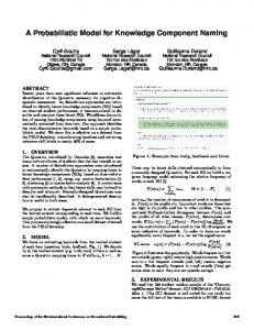
Figure 2. Segmentation of synthetic image in CIELAB. Upper left Original image, upper right PLSApg model, middle right ML-training set of 11 terms, middle left MAP-training set of 11 terms, low left MLtraining set of 47 terms and low right MAP-training set of 47 terms.

Image Quantization Extracting the perceived color from an image can operate in a similar way to various quantization algorithms for data reduction. The first step was to test the performance of both models with a basic and an extended training set to segment the synthetic image used by a recent published color-naming algorithm [29], shown in Fig. 2 and 3. The coordinates of their centroids in the experimental data were used to color each color category of both models. Although the challenging synthetic image consisted of a continuous gradation of highly saturated colors in various lightness levels, both algorithms successfully classified the total number of pixels without artifacts at the borders. In terms of implementation, both models offer computational simplicity and fast performance. Specifically MAP can be computed with one extra matrix multiplication and for a single CIELAB triplet requires only 9.6% more processing time than ML. A summary of color naming statistics is presented in Fig. 4 and Fig. 5 to provide an insight about the principal color names identified in the image for ML and MAP with an extended training set. Figure 3 Synthetic image in CIELAB.

Figure 4. Summary of color naming statistics of synthetic image using ML estimator.

Using the ML approach, the synthetic image was segmented into 30 categories whilst the MAP method favored 20 color names in wider cultural use. Restricting the training set to basic color terms produced misleading color identifications, for example an area identified as brown was named as tan or beige by the majority of our observers. The cognitive representation of statistical regularities of natural images can be used to encode them more efficiently, since color-naming algorithms can combine neighboring regions that share the same cognitive color concept. Fig.6 shows the performance of ML and MAP models in image segmentation of natural images. The segmentation of natural images showed that the ML approach produced better results for users with a non-basic color vocabulary, since the favoring of more frequent color names of MAP resulted in the loss of important face information and caused a large area of burgundy to be classified as brown on the poppies.

Discussion, Conclusions and Future Plans We have presented a flexible color naming architecture for automatic assignment of color coordinates to color names based on Maximum Likelihood and Maximum a Posteriori estimators. The strength of our methodology lies in the fact that both algorithms can operate online with a large database of a web-based color naming experiment with important additional information. This allows the training set to be adapted to the color vocabulary of the users. The evaluation of the models showed that the goodness of fit of the parameters predicted by ML was slightly better than that provided by MAP, however the precision of the latter was more consistent on both sets. Given that both algorithms were evaluated on grids, a possible explanation for the errors could be the replacement of the conditional probabilities with their normal approximations. However, the smoothed categories stabilized the classification procedure, which is an important requirement in imaging applications. In addition, the comparison of the predicted color categories with rigorous psychophysical studies resulted in a

Figure 5. Summary of color naming statistics of synthetic image using MAP estimator.

significant improvement than we had previously reported. The superiority of ML in segmenting natural images indicates the need to select the model according to the application. However, the question, whether we prefer MAP or ML approach, is equivalent to whether we take into account that color names are used equally or not. Both models appear to be suitable for online applications, given their computational simplicity and fast performance. Further work is still needed to develop a comprehensive online color-naming model, including psychophysical validation of the performance of the model and investigation of the distribution of the extended color vocabulary. Given that each color name is associated with specific categorical viewing conditions in the color naming dataset, the next step should be the improvement of the model to compensate for color appearance issues. Differences between responses according to language, age and gender will also be investigated. On the World Wide Web color specification is not only the domain of experienced color users, but is a facility required by large audiences with a need to communicate about color out of their local physical environments. The ongoing study reported here has made a practical contribution to color communication within different cultures.

Acknowledgements The authors would like to acknowledge Dr Jason Chuang at Stanford University and Dr Maureen Stone for their help towards the implementation of the probabilistic model of categorical association, Dr Michael Studer for his comprehensive comments regarding the statistical analysis, and Dr Nathan Moroney at HP Labs for having made available the Radial OSA data and opened the way for online chip-based experimental methods. This work has been partially supported by TruColour Ltd.

References [1] [2]

Benavente, R. (2005). A parametric model for computational colour naming. PhD Thesis. Universitat Autonoma de Barcelona. Benavente, R., Vanrell, M. and Baldrich, R. (2008). Parametric fuzzy sets for automatic color naming. J. Optical Society of America A, 25(10), 2582-2593.

(i) (ii) (iii) (iv) (v) Figure 6. Image segmentation of natural images using ML and MAP estimators. (i) Original image, (ii) ML-training set of 11 terms, (iii) MAP- training set of 11 terms, (iv) ML- training set of 47 terms and (vi) MAP- training set of 47 terms.

[3]

Berlin, B. and Kay, P. (1969). Basic color terms: their universality [19] Mojsilovic, A. (2005). A computational model for color naming and and evolution, Stanford, Calif.: Center for the Study of Language and describing color composition of images. IEEE Trans. on Image Information. Processing, 14(5), 690-699. [4] Boynton, R.M. and Olson, C.X. (1987). Locating basic colors in the [20] Moroney, N. (2003a) A Radial Sampling of the OSA Uniform Color OSA space. Color Research & Application, 12(2), 94-105. Scales. Proc. IS&T/SID 11th Color Imaging Conf., 175-180. 4.A.Image segmentation natural images using and MAP estimators. Original [5]Figure Chapanis, (1965). Color names for colorof space. American [21]ML Moroney, N. (2003b). Unconstrained(i) web-based color image, naming 53, 327-346.set of 11 terms, (iii) MAP-learning set of experiment. Proc.(iv) SPIE ML-47 Conf. on Color Imaging Processing, (ii)Scientist, ML-learning 11 terms, terms andVIII: (vi) MAP[6] Chuang, J., Hanrahan, P. and Stone, M. (2008). A Probabilistic Model Hardcopy, and Applications, 5008, 36-46. learning set of Association 47 terms. of the Categorical Between Colors. Proc. 16th IS&T/SID [22] Moroney, N., Obrador, P. and Beretta, G. (2008). Lexical Image Color Imaging Conf., 6-11. Processing. Proc. IS&T/SID 16th Color Imaging Conf., 268-273.. [7] Davidoff, J., Davies, I. & Roberson, D. (1999) Color categories of a [23] Motomura, H. (1997). Categorical Color Mapping for Gamut stone-age tribe. Nature, 398, 203-204. Mapping. Proc. 5th IS&T/SID Color Imaging Conf. 50-55. [8] Derefeldt, G. and Swartling, T. (1995). Colour concept retrieval by [24] Mylonas, D. and MacDonald, L.W. (2010). Online Colour Naming free colour naming. Identification of up to 30 colours without Experiment using Munsell Colour Samples. Proc. 4th Eur. Conf. on training. Displays, 16(2), 69-77. Colour in Graphics, Imaging and Vision (CGIV), 27-32. [9] Derefeldt, G., Berggrund, U. and Swartling, T. (2004). Cognitive [25] Mylonas, D. and MacDonald L.W. (2009). Online Colour Naming color. Color Research & Application, 29(1), 7-19. Experiment, Available online at: http://colornaming.net [10] Franklin, A., Drivonikou, G.V., Bevis, L., Davies, I. R. L., Kay, P., [26] Sparacino G. et al. (2000) Maximum-Likelihood versus Maximum a and Regier, T. (2008). Categorical perception of color is lateralized to Posteriori Parameter Estimation of Physiological System Models: The the right hemisphere in infants, but to the left hemisphere in adults. C-peptide Impulse Response Case Study, IEEE Trans. on Biomedical Proc. National Academy of Sciences, 105(9), 3221-3225. Engineering, 47(6), 801-811. [11] Frascara J. (1997). User-Centred Graphic Design. Mass [27] Sturges, J. and Whitfield, A. (1995). Locating basic colors in the Communications and Social Change. Taylor & Francis, Great Britain Munsell Space. Color Research and Application, 20(6), 364-376. [12] Gage, J. (1993). Color and culture : practice and meaning from [28] Tan, L.H. et al. (2008). Language affects patterns of brain activation antiquity to abstraction, Boston: Little, Brown and Company. associated with perceptual decision. Proc. National Academy of [13] Green P. (2002) Colorimetry and colour difference, in Green, P. and Sciences, 105(10), 4004-4009. Macdonald, L.W., Colour Engineering. UK: John Wiley [29] Weijer J., Schmid C., and Verbeek J. (2009). Learning Color Names [14] Kaiser, P.K. and Boynton, R.M. (1996). Human color vision, from Real-World Images. IEEE Trans. on Image Processing, 18(7). Washington, DC: Optical Society of America. [30] Woolfe, G. (2008). Natural Language Color Communication and [15] Lammens, J. (1994). A computational model of color perception and System Interface. US Patent Application US2008/0007749. color naming. PhD Thesis. State University of New York at Buffalo. [16] Lin, H., Luo, M.R., MacDonald, L.W. and Tarrant, A.W.S. (2001c). A cross-cultural colour-naming study. Part III – A colour-naming Author Biography model. Color Research & Application, 26(4), 270-277. Dimitris Mylonas received his MSc in Digital Colour Imaging from [17] MacDonald, L.W. (1999) Using color effectively in computer the London College of Communication, University of the Arts (2009). He is graphics, IEEE Computer Graphics and Applications, 19(4), 20-35. currently working at the University of Liverpool and TruColour Ltd. His [18] MacDonald, L.W. and Mylonas, D. (2010) Edible Color Names, work focuses on visual communication design and color management Proc. AIC 2010 Conf. on ‘Color and Food’, Mar del Plata, Argentina, solutions in web based environments. He is a member of IS&T, SDC and October 2010. Colour Group GB.