Graphic Arts in Finland 35(2006)2
Color Naming and Computational Prediction from Natural Images Nurminen, T*, Kivinen, J.**, Oittinen, P.*** Helsinki University of Technology, Department of Automation and Systems Technology, Media Technology Laboratory P.O.Box 5500, FIN-02015 HUT, Finland, http://www.media.tkk.fi E-mail:
[email protected],
[email protected],
[email protected] * Master's thesis student, ** Instructor, *** Supervisor
ABSTRACT The article at hand is based on the master's thesis by one of the authors entitled "Color Naming and Computational Prediction from Natural Color Images" /21/. The work was conducted in the Laboratory of Media Technology at Helsinki University of Technology under the supervision of Professor Pirkko Oittinen and the instruction of Jyri Kivinen M.Sc.. The objective of the work was to develop a format for describing color information of digital images based on quantitative measures. The purpose of the proposed format was to serve the needs of the image production chain concerning various processes and related communication. The emphasis was on image retrieval and image selection. The principal aim was to support Finnish production teams. A method was developed for describing the dominant colors of natural images using linguistic expression. The method was based on the dominant color descriptor of the MPEG-7standard and it utilized ISCC-NBS color vocabulary for the linguistic conversion of the color values. Three experiments were conducted in order to gain information for constructing a modified version of the ISCC-NBS vocabulary and to test the method for naming dominant colors from images. The results proved that the dominant colors produced by the color naming method correspond well with human responses within limits of similarity among color names, even though some shortcomings were registered. The developed color vocabulary was, however, estimated to be too detailed for its purpose.
INTRODUCTION In the first section some of the most relevant background on which the study is based is presented. The research area to which the study is strongly connected is image retrieval research. Therefore some of the important aspects related to the research field are outlined. The objects of the study are presented at the end of the section. The follow-up of the article consists of three sections. The first section, carrying the title Research Methods and Data, presents the computational method for computing the color description as well as the design of the experiments. Furthermore the methods used for analyzing the data gained from the experiments are described. In the second section the results of the experiments are evaluated. The last section contains the discussion concerning the study as a whole.
13
Graphic Arts in Finland 35(2006)2 Image Retrieval Research We have witnessed a rapid growth in the quantity of digital images, which shows no signs of abating The phenomenon has created a demand for developing new ways of tackling the challenge of managing digital image databases. There is a need for creating tools for supporting image retrieval, browsing, and selection. A whole new research field has emerged from this need. The research area has been very active for over two decades but it has still not been able to attain the goals that were set for it. There remain a vast number of questions that need to be answered. Many hopes placed on the matter are still to be achieved. Image database searches have been based on metadata linked to images. Metadata can hold a description of the corresponding image with varying fields. Traditionally, metadata has been manually fed to a database. This approach is not satisfactory as it requires a huge amount of tiresome work and is error prone as well as inaccurate. The task of producing the metadata manually becomes more and more laborious especially as the revolution of digital imaging has explosively increased the number of images. That is why an aim evolved to automatically produce metadata that describes the image related to it. This has been done to this day by computationally extracting typically low-level information from raw image data. The approach is called content-based image retrieval. However, the research soon ran into a problem, nowadays commonly known as semantic gap. The concept refers to the gap between the low-level information that is possible to be extracted quite robustly from the image data and the high-level concepts that people attach to images. The term semantic refers commonly to the meaning of words. For a lengthy period of time the research has focused on bridging the semantic gap. Some promising solutions have been presented over the years but still the work is far from complete. Therefore, it is no surprise that the research field is very active indeed. For extensive overview of content-based image retrieval research see /22/. Content-based image retrieval commonly requires the search task to be conducted using query by example or query by sketch approach as an option for text-based search, e.g. /23,25/. In this situation the system returns images that are most similar to the example image or sketch. Another approach is that the system first offers a set of images from which the user selects the most relevant ones. Then the search is iteratively refined according to user feedback. This method is called relevance feedback, e.g. /11/. It may also be assumed that the methods presented follow a text-based query. All approaches serve a purpose in developing systems that are adaptable to the variety of user needs. Still, the importance of language in image retrieval systems is often ignored even though there has been a fair amount of research concerning language based query, e.g. /24/. Since categorization is originated from language it is self-evident that support for different languagebased search tasks is needed. Language can be seen as the key to the semantics of images. Research Objective The overall objective for the study was to develop a format describing color information of digital images. The purpose of the format was to serve the needs of image production chains involved in various processes. The aim was primarily intended to promote Finnish production teams. The emphasis was specified to be on image retrieval and image selection. In addition, it was stated that communication among actors in the image production chain would be taken into account. Finally, it was determined that the representation of color information based on quantitative measures would be visually verified.
14
Graphic Arts in Finland 35(2006)2
More precisely the aim of the master's thesis was to develop a method for computationally extracting color information from natural images and converting it to a form that would fulfill the requirements.
RESEARCH METHODS AND DATA As mentioned above the aim of the research was to develop a format for describing color information of natural images in order to promote the work flow of image production chains. For this purpose a method for naming dominant colors from natural images was established and a set of experiments with test subjects were conducted in order to test the method. In this section the method for naming dominant colors from natural images is presented. The experiment design is also described as well as the methods used to analyze the data gathered from the experiments. The Dominant Color Naming Method Based on a literary survey had been conducted the MPEG-7 standard /4,5,6/ was placed under specific examination. The MPEG-7 includes four color descriptors for describing the color information in images. The color descriptors include color layout, color structure, scalable color and dominant color descriptor. The MPEG-7 color descriptors have been put to use in image retrieval, for example /11,12,13/. The last named was chosen for describing the color information on the dominant color descriptor of the MPEG-7 standard. The reason behind the decision was the fact that one of the goals was to promote communication among actors in the image production chain. Therefore, linguistic description was seen as a requirement for expressing the color information. The dominant color descriptor was regarded as most suitable for the purpose, due to its simple form. Next, a short description of the structure of the MPEG-7 dominant color descriptor is given as well as the basic steps for forming it. The MPEG-7 dominant color descriptor consists of maximally eight colors for which the following characteristic values are given: center in RGB-values, percentage of related pixels compared with all pixels in the image, variance and spatial homogeneity. Briefly described, the dominant color clusters are generated by applying peer group filtering /7/ to the image. Then, dominant color clusters are formed using k-means -clusterin /9, pp. 50-51/, followed by agglomerative clustering /10, pp. 552-553/, which connects clusters with centroids that are closely located in the color space. Peer group filtering also generates perceptual weights that are used in the clustering. The weights are calculated taking into account the neighborhood of the pixel, since the human visual system is more sensitive to changes in smooth areas than in textured areas in the image /7,17/. The clustering method at hand is a variant of the k-means algorithm. K-means algorithm can be used to find K representative clusters and their centroids from data given initial positions of the centroids and a stopping criterion. The number of the clusters is fixed to K along the iterations of the algorithm. The clustering method at hand proceeds as follows. First the mean of the data is computed and a centroid is allocated to that position. Then the data cluster is partitioned into two clusters. The
15
Graphic Arts in Finland 35(2006)2
cluster centroids are initially chosen with the help of principal component analysis (PCA) of the cluster data. The coordinates of the new centroids are chosen to be a defined distance apart (that is relative to the variance of the cluster data) along the first principal axis, from the centroid of the cluster that was split, to opposite directions. The coordinates of the new centroids are chosen to be a defined distance apart (that is relative to the standard deviance of the cluster data along the first principal axis), from the centroid of the cluster that was split, to opposite directions along the first principal axis. K-means clustering minimizes sum of squares error (SSE) and the first principal component direction produces the largest SSE. Therefore that direction is a good candidate for projection in order to partition the cluster. Then two steps of k-means learning rule, assigning each data point to a centroid according to nearest neighbor rule and updating the centroids, are repeated until the termination rule (in this case maximum amount of iterations) is fulfilled. Next the cluster which has the largest sum of squares error is chosen as the next cluster to be partitioned and PCA is used in defining the two new initial centroids as before. After the number of clusters has incremented by one the data points are assigned to clusters and centroids are updated once again by k-means. This procedure is repeated until the defined number of clusters has been attained. Assigning initial centroids by using PCA has been empirically proven to give close to minimum the error sum of squares values. In which case the minimum values are produced by selecting the best performance from a hundred randomly initialized runs. In addition the empirical evidence states that less iteration steps are needed than with methods using random initialization. For more details see /18/. Linguistic conversion of the color values produced by the dominant color descriptor was done using the modified ISCC-NBS vocabulary /8,14/ of 267 color names. This particular vocabulary was chosen due to the fact that it was developed by an official institute formerly known as The National Bureau of Standards, nowadays referred to as The National Institute of Standards and Technology. The other cogent reason was that few well-defined color vocabularies were available. Formerly, Mojsilovic /2/ had used the ISCC-NBS vocabulary in her research. Most image retrieval methods that involve actual color names use the basic color terms developed by Berlin and Kay /3/. The eleven basic color terms are red, blue, yellow, green, orange, purple, pink, brown, gray, white, and black. However, it was estimated that by using the basic color terms the color information of natural images could not be described with the requisite precision considering the nature of the context. The decision was based on the literary survey which indicated that people tend to use modifiers for saturation and brightness when freely describing color names related to natural images, for details see /2/. The third level of the ISCC-NBS vocabulary (which initially consisted of 267 color terms) was narrowed down to 230 color names. The vocabulary was then translated into Finnish. The vocabulary was defined as areas in the Munsell color system /15/. The color centers of the corresponding color names were defined as the approximated centers of the Munsell color areas. The centers were then converted to Lab color space. The attachment of the color names to the color values produced by the earlier phase was done by calculating the Euclidean distances of certain color values to the color centers defined by the vocabulary and selecting the name with the shortest distance to the color value. The operation was performed in Lab color space because of its perceptually uniform nature. The algorithm is more closely represented in Figure 1 as a flow chart.
16
Graphic Arts in Finland 35(2006)2
Figure 1
The Dominant Color Naming Algorithm represented as a flow chart.
Experiments and Methods Used for Data Analysis Next the three test subject experiments are introduced. At the end of this section hierarchical clustering method is described, since it was used in analyzing the data of the third experiment of naming dominant colors from images. In the original study also other methods such as
17
Graphic Arts in Finland 35(2006)2
multidimensional scaling and confusion matrix were used. These methods are not described since the analyses related to these methods are not presented in this article either. The experiments were conducted in order to obtain information to construct the color vocabulary used in the dominant color-naming algorithm and in order to evaluate the performance of the algorithm. In all three experiments there were thirty test subjects. All were students at the University of Technology. All the test subjects had Finnish as their native language. Eight of the subjects were female and twenty-two were male, their ages ranging between eighteen and twenty-eight years. Ishihara's color blindness test /1/ was conducted on all of the test subjects before the tests. The first and the second test were executed on the same occasion. The test room was lighted with fluorescent lamps of 3000 kelvins and 28 watts. The illuminance level of the ViewSonic monitor was approximately 465 lux. There was no time limit on any of the tasks in the experiments. First Experiment: Color Listing In the first experiment the test subjects were asked to write down at least eleven important color names. The subjects were advised to write down only names that were monolexic. Moreover, they were not allowed to choose color names that referred to objects. The goal of the color listing test was to evaluate how common the corresponding basic color terms first presented by Berlin and Kay are in the Finnish language. Also, the aim was to estimate the frequency of color hues that appear in the ISCC-NBS color vocabulary [8]. The experiment corresponded to the test presented by Mojsilovic /2/. The test-related results presented by Mojsilovic supported the impression of the test being suitable for the purpose. Second Experiment: Color Naming Using Vocabulary In the second experiment the test subjects were presented with the patches corresponding to the 267 color centers of the built-up color vocabulary, one at a time on the monitor. The patches were the size of 200x200 pixels on a light gray background. The test subjects were asked to name the patches using the color vocabulary. The color vocabulary consisted of 230 color names; therefore a few color names were represented by more than one center. The aim of the second experiment was to verify the ISCC-NBS color vocabulary /8/, or, more precisely, to examine how well the names attached to the color patches by the test subjects corresponded to the names of the color centers presented by the vocabulary. Thus the goal was to obtain a view of the usability of the vocabulary concerning color naming applied to the task at hand. Third Experiment: Naming the Dominant Colors from Images The aim of the third experiment was to test how well the implemented algorithm performed. For that purpose forty natural color images were selected from Kodak's CD so that the images represented had different motifs and varying colors. The images were presented on a monitor to the test subjects one at a time. The test subjects were asked to list the dominant colors of the images by name, using the color vocabulary. The subjects were advised that the number of dominant colors was to range from one to eight, as the range is the same in the MPEG-7 dominant color descriptor.
18
Graphic Arts in Finland 35(2006)2 Hierarchical Clustering Hierarchical clustering was used to compare the results of the dominant colors named by the test persons from forty images in the third experiment and the dominant colors produced by the implemented algorithm given the same colors as input. For this purpose the test persons' data was converted to binary form by turning the colors that more than 13.33 percent of the participants had named to 1 and the others to 0. Then separated distance matrices were formed from the data. The distance between two images was calculated by adding together the color difference between each color and the closest color belonging to the other image being compared and dividing the sum by the total number of colors. Hierarchical clustering was performed by using incremental approach and complete linkage.
RESULTS AND DISCUSSION First Experiment: Color Listing In the color listing experiment all thirty subjects named only eleven colors which was the minimum. The test subjects used quite a short time to perform the task even though no time limit had been set. Some test persons seemed to experience anxiety over the fact that they did not seem to remember relevant colors although they had the feeling that some important colors were missing. These two facts perhaps explain some of the somewhat surprising results. All test subjects had included red, blue, yellow, and black in their list of most important colors. Most test subjects, at least 80 percent of them, had also included green, orange, white, and gray in their list. It was perhaps rather surprising that not all the test subjects had named green. In addition, many of the subjects, in the range of 50 to 77 percent, had added violet, brown, and turquoise to their list. Only 30 percent or fewer of the test subjects had named the following colors: light red, (monolexic in Finnish, can also be translated as pink) lilac / mauve, beige, magenta, cyan, and purple. The full results of the experiments are presented in Table 1.
19
Graphic Arts in Finland 35(2006)2
Table 1 Color name
Results of the color naming experiment. Amount of named
Percentage
red
30
100.0
blue
30
100.0
yellow
30
100.0
black
30
100.0
green
29
96.7
orange
29
96.7
white
27
90.0
gray
24
80.0
violet
23
76.7
brown
23
76.7
turquoise
17
56.7
light red (pink)
9
30.0
lilac
7
23.3
beige
6
20.0
magenta
6
20.0
pink
4
13.3
cyan
4
13.3
purple
2
6.7
When compared with the basic color terms proposed by Berlin and Kay /3/ some relevant observations can be made concerning the special characteristics of the Finnish language. In the light of the results the most problematic color terms were light red / pink (vaaleanpunainen), pink (pinkki), and purple (purppura). None of the colors had received more than ten votes. Only two of the participants had included purple in their list. On the other hand, twenty-three subjects had name violet (violetti). Purple is one of the basic color terms of Berlin and Kay. However, it can be presumed that the role of the term is less prominent in Finnish. The role of lilac as a basic color term is more plausible and therefore a good candidate for use as a hue name in the vocabulary. The low frequency of light red and pink casts doubt on their presence in the dictionary. Moreover, the monolexic nature of light red is questionable even though it is a compound. However, light red was chosen for inclusion in the dictionary because it was felt that one of the terms needed to be included as the term pink was well represented in the ISCC-NBS color vocabulary. All the color names that more than half of the participants had named were basic color terms of Berlin and Kay with one exception: turquoise. Therefore its role as a basic color term should be considered. The research done by Taft and Sivik /16/ would also support the fact. Nevertheless it was left out of the vocabulary as its occurrence frequency was not particularly high. Also, it should be noted that none of the participants named olive as a color name although it appeared in the ISCC-NBS vocabulary. That is why the name was replaced by the term brownish green (ruskeanvihreä) in the modified vocabulary.
20
Graphic Arts in Finland 35(2006)2 Second Experiment: Color Naming Using Vocabulary In the second experiment the test subjects used the modified ISCC-NBS vocabulary /8/, consisting of 230 color terms, to name color patches which represented the center points of the corresponding color names in the vocabulary. Only the most relevant results gained from the data are presented next. The data concerning the second experiment were scattered. The standard deviation of color difference (∆ E) among the test subjects, when all answers were considered, was 16.5 units. On average 3.6 subjects out of thirty participants, that is 11.9 percent of the respondents, named the presented color patch as the same color as the color centers related to the vocabulary. The color differences in the answers of the subjects and the color names presumed by the color vocabulary were investigated. In other words, with every patch the Euclidean distance in Lab color space was calculated between color centers of the color names given by respondents as they were listed in the color vocabulary and the color center specified by the vocabulary. From the distances obtained the percentage of the calculated distances that were under a given threshold value was investigated. More than 52.2 percent of the distances were under the threshold value of twenty units. For comparison, the color names bright blue (kirkas sininen) and strong blue (voimakas sininen) were situated at a distance of twenty units in the Lab -color space according to the vocabulary. Applying the threshold value of sixty units, most of the distances calculated from the data, i.e. 98.8 percent, fall under the threshold. For example, the distance between bright yellowish green (kirkas keltavihreä) and strong green (voimakas vihreä) was close to sixty units. The histogram visualizing the distribution of the distances is presented in Figure 2.
Figure 2
Histogram of Euclidean distance between the vocabulary colors and the test subject answers (horizontal axes: Euclidean distance, vertical axes: the percentage of answers).
21
Graphic Arts in Finland 35(2006)2
All colors taken into account, the average distance between the answers and expected colors was 20.4 units. The test subject answers matched the vocabulary best with achromatic colors, quite expectedly. Chromatic colors that gave good matches (with a threshold value under 10 units) were bright yellow (kirkas keltainen), bright red (kirkas punainen), light blue (vaalea sininen), light red / pink (vaaleanpunainen), pale red / pale pink (haalea vaaleanpunainen), dark blue (tummansininen), dark violet (tummanvioletti), very dark green (hyvin tummanvihreä) and grayish dark blue (harmahtava tummansininen). A clear pattern could not be observed from the color names. Notably weak performance was found with certain shades of green and yellow. The very worst results (with average distance of over forty units) received with the following colors bright yellowish green (kirkas keltavihreä), bright greenish yellow (kirkas vihreänkeltainen), strong yellowish green (voimakas keltavihreä), strong greenish yellow (voimakas vihreänkeltainen), deep greenish yellow (syvä vihreänkeltainen), dark greenish yellow (tumma vihreänkeltainen), and bright bluish green (kirkas sinisen vihreä). One reason for the poor performance of the different shades of yellowish greens and greenish yellows could be the fact that there is no color name between yellow and green. Even though yellow, red and blue are sometimes considered to be primary colors, at least the human visual system supports the idea of green being a primary color as well. However, there is not a secondary color between yellow and green that would have a well established name, as every other primary color has, although turquoise did not appear as a hue name in the vocabulary. The color term lime could be suggested as a solution. However, the role of lime as a color name is problematic since it is not an established term. The distances between the average answers of the test subjects and the defined vocabulary color centers are visualized in Figure 3.
Figure 3
The vocabulary colors shown as points in a- (green-red) and b-axes (blue-yellow) of Lab -color space. The size of the point represents the distance between the average distance of test subject answers and the defined color center so that a smaller point corresponds to a smaller distance.
22
Graphic Arts in Finland 35(2006)2
When analyzing the most frequently occurring colors, it was discovered that bright primary colors and monochromatic colors as well as different shades of blue were used most repeatedly. It was also noted that the test subjects used short color names more frequently than long ones with preferably only one prefix describing the saturation or brightness of the color or non-dominant hue in addition to the main hue name. Furthermore, some observations were made while comparing the names of different color centers assigned by the vocabulary and the color names that the participants most frequently gave to the shown color patches. With expected hue name of brownish green (ruskeanvihreä) clearly most popular answer was dark green (tummanvihreä). As already mentioned, yellowish greens (keltavihreä) and greenish yellows (vihreänkeltainen) were mixed together. Quite a few green (vihreä) colors were perceived as bluish green (sinisenvihreä). On the other hand, colors named in the vocabulary as greenish blue (vihreänsininen) were labeled as blue (sininen) by the test subjects. In addition, colors that in the vocabulary went by the name of purplish blue (purppuransininen) were mostly named simply blue (sininen) as a hue name. A somewhat interesting observation was that purple (purppura) hue names appearing in the vocabulary were most frequently named violet (violetti). Also, hue names with two parts, such as reddish purple (punaisenpurppura) and purplish pink (purppuranvaaleanpunainen), were simply named purple (purppura) and pink (vaaleanpunainen) respectively. Moreover, the participants labeled a rather peculiar color name yellowish pink (keltaisenvaaleanpunainen) most frequently as orange (oranssi). Third Experiment: Naming the Dominant Colors from Images In the third experiment the participants named the dominant colors in forty images using the modified ISCC-NBS -vocabulary /8/. The maximum number of dominant colors per image was set at eight. The dominant colors from the same images were determined also using the implemented algorithm described earlier. After these procedures the results were compared. The algorithm produces color names ranging from three to eight per image as the test subjects named colors ranging from three to six per image. The average number of colors produced by the algorithm was seven and the average with test subjects was four. Thus the algorithm generally produced more colors per image than the test subjects did. In view of the results, it should be considered that the maximum number of colors would be set at six and that the parameters of the algorithm would be tuned so that they would produce fewer dominant colors overall. The fact that even though the average number of dominant colors per picture named by a test subject was four, and that the average of different color names per picture was forty-three, when considering all the answers, gives an idea of the amount of scattering among the answers. The number of color names that more than half of the subjects had named from one specific image was on average only one. However, it should be noted that the color name black (musta), which was quite coherently named, raised the average. The results were analyzed using hierarchical clustering as presented in the main section Research Methods and Data under the heading Hierarchical Clustering. As the image group used in the experiment consisted of only forty samples, only two clusters were formed. Comparison of the two clusters, one with results attained using the algorithm and the other from the test subject data, showed that the clusters were seventy-five percent alike. In general, the images in the second cluster had bright, warm colors. Very specific characteristics concerning unity inside the clusters and the difference between clusters could not be defined since the number of images, and therefore the number of clusters, were so few.
23
Graphic Arts in Finland 35(2006)2
A comparison was made by analyzing the color difference in Euclidean distance in Lab -color space among all the colors named by the test persons and the closest color produced by the algorithm, image by image. It was revealed that over sixty percent of the named colors were closer than thirty units in distance. The result can be considered excellent when compared with the fact that in the second experiment, when patches were named, the average distance between named color and the color offered by the vocabulary was 20.4 units. In the master's thesis a comparison based on visual presentation was also made among the dominant colors produced by the algorithm and the test person data, image by image. In general, it can be stated that the algorithm did not produce colors that the test subjects had named if the area of the color in the image was small. With some images, the colors that the algorithm had produced were clearly less saturated and less bright than the colors the subjects had named. One explanation for this phenomenon is that the color names in the vocabulary are perceived as being less saturated and less bright than those defined according to the vocabulary. Another explanation is the fact that the human perception of the image differs notably from the stored image information. Even though in the algorithm there existed a part that calculated the perceptual weights for the pixels, it was not sufficient to model the perception of the human visual system. The algorithm, for example, regards the shadow areas in the images, whereas humans in many cases discard the different shades of color in the shadows. The Euclidean distance proved to be inadequate since the distortion in the conversion process to color name was in some cases excessive, though preferable, due to its simplicity. Two examples of good and poor algorithm performance are represented respectively in Figure 4 and Figure 5. The test images are on the right hand side. The dominant colors produced by the algorithm are visualized on the left in the upper row. The colored proportion of the bar corresponds to the percentage of the pixels belonging to the cluster compared to all the pixels in the image. The test subject answers are presented on the left hand side in the lower row. The answers are separately grouped under the dominant color of the algorithm which is the closest in Euclidean distance. Therefore the colored proportion reflects the number of answers. It can be seen from the bars in Figure 4 that the dominant colors produced by the algorithm correspond quite well with the answers given by the test subjects. In the case of the first image with the elephant also the proportions of the colors match fairly well. On the other hand, looking at Figure 5 it can be noticed that some of the colors produced by the algorithm match poorly with the test subject answers. In the case of the first image with light pink flowers test subjects have frequently named shades of dark green and bright pink. Still, the algorithm has not produced greens and the shades of pink are light. The fact that there is no green in the dominant colors of the algorithm could perhaps be explained by the fact humans probably perceive mainly the bright areas from the image as the algorithm takes note of the shady areas as well as mentioned earlier. The bright pink versus light pink problem is more likely to be at least partly the consequence of the fact that the colors attached to the color names differ from the colors specified by the vocabulary. With the bottom image in Figure 5 with the yellow flower the assumption is that the reason for yellow not occurring as a computed dominant color even though there are the shades of yellow in the subject answers is the same as before. That is to say that the algorithm does not give more weight in bright areas and therefore averaging produces darker shades than humans perceive.
24
Graphic Arts in Finland 35(2006)2
Figure 4
Two examples of good algorithm performance, on the right the test images and on the left, upper row: dominant colors of algorithm, lower row: test subject answers.
25
Graphic Arts in Finland 35(2006)2
Figure 5
Two examples of poor algorithm performance, on the right the test images and on the left, upper row: dominant colors of algorithm, lower row: test subject answers.
CONCLUSION In this study a method for naming dominant colors from natural images was presented. The method at hand was composed of an applied dominant color descriptor of the MPEG-7 -standard /4,5,6/ and a conversion procedure of color centers to color names that uses a revised ISCC-NBS vocabulary /8/ translated into Finnish. In the experiments conducted with test subjects, the implemented method proved to be promising. The results of the experiments showed that the dominant colors produced by the algorithm corresponded well with human responses within the limits of similarity between color names, even though shortcomings were also registered. The results of the second experiment indicated that the color vocabulary used was too precise, as the attachment of the color names to certain values in the color space was very subjective. On the other hand, the assumption is that the basic color terms of Berlin and Kay are too broad to be useful, for example for use by image production staff in a magazine, even though they are widely used in image retrieval research. One challenge is to connect the developed color vocabulary to a color space. Several methods have been proposed, for example /2,19,20/. However, most of the research has been based on color categories of the eleven basic color terms. The clustering part of the method should be further developed to correspond better to the color perception of humans concerning natural images. One of the major drawbacks of the clustering
26
Graphic Arts in Finland 35(2006)2
was that it was continued until there were a maximum of eight color clusters. The use of a small number of clusters resulted in color centers that were too averaged. On the other hand, it was necessary that the method produced only a small number of dominant colors, as the experiment with test subjects proved. Therefore the model should be revised. A suggestion for the outline of a new approach is that the clustering be terminated earlier and the produced color clusters would then serve as candidates for final dominant colors. The final dominant colors would be chosen from the candidates, using different criteria. The criteria could for example be size, spatial coherence, and salience of the color. Shape and texture information could also be used for the purpose. In addition, an interesting topic for further research would be to investigate the connection of colors to the impression of the image. This would involve approaching images on a higher semantic level. In the future, the method for naming dominant colors could be used as part of the digital stripping table and of the image agent that functions as an engine of the system. The ability to define the dominant colors of an image could be used as a modifier in search tasks as well as in the presentation of a group of images in the task of selecting and browsing. The color vocabulary is also connected to semantic web-related ontologies. In order for a colorname ontology to be functional it should incorporate relevant concepts and feelings that people apply to colors. In the ontology, assertions such as "red, yellow and orange are warm colors", "green is the complementary color of red" and "violet is close to blue" should be explicitly formulated.
REFERENCES 1.
Ishihara, S,. Ishihara Test for Color Blindness. Kanehara Shuppan, Tokyo, Japan 1969.
2.
Mojsilovic, A., A Method for Color Naming and Description of Color Composition in Images. Proceedings in International Conference on Image Processing, Rochester, New York, USA, September, 2002, pp. 789792.
3.
Berlin, B., Kay, R., Basic Color Terms: Their Universality and Evolution. Berkeley: University of California, San Franscisco, USA, 1969.
4.
Manjunath, B. S., Salembier, P., Sikora, T., Introduction to MPEG-7 - Multimedia Content Descriptor Interface. John Wiley & Sons, Ltd., Chichester, England, 2002. ISBN 0-471-48678-7.
5.
Cieplinski, L., MPEG-7 Color Descriptors and Their Applications. Lecture Notes in Computer Science, 2001, vol. 2124, pp. 11-20, ISSN: 0302-9743.
6.
Cieplinski, L., Kim, M., Ohm, J.-R., Pickering, M., Yamada, A., (Eds.) Texts of ISO/IEC 15938-3/FCD Information Technology - Multimedia Content Description Interface - Part 3: Visual. ISO/IEC JTC1/SC29/WG11 (MPEG) document no. N4062, Singapore, SG, March 2001.
7.
Deng, Y., Kenney, C., Moore, M. S., Manjunath, B. S., Peer Group Filtering and Perceptual Color Image Quantization. Proceedings of IEEE International Symposium on Circuits and Systems VLSI, Orlando, Florida, USA, June 1999, vol. 4, pp. 21-24.
8.
Kelly, K., Judd, D., The ISCC-NBS Color Names Dictionary and the Universal Color Language. NBS Circular 553, November 1, 1955.
9.
Kung, S. Y., Mak, M. W., Lin, S. H., Biometric Authentication. A Machine Learning Approach. Pearson Education, Inc., New Jersey, USA, 2004. ISBN 0-131-47824-9.
10. Duda, R. O., Hart, P. E., Stork, D. G., Pattern Classification. (Second Edition) John Wiley & Sons, Inc., New York, USA, 2001. ISBN 0-201-63464-3. 11. Koskela, M., Laaksonen, J., Oja, E., PicSom - Self-Organizing Image Retrieval with MPEG-7 Descriptors. In Proceedings of Infotech Oulu International Conference on Image Retrieval. Oulu, Finland. September 2001.
27
Graphic Arts in Finland 35(2006)2
12. Sert, M., Alpay, M., Çakir, B., Content-Based Image Retrieval of Medical Images in MPEG-7 Databases. IJCI Proceedings of International Conference on Signal Processing, September 2003, vol. 1, no. 2, ISSN 1304-2386. 13. Suroung, S., Liang-Tien, C., Rajan, D., Efficient Image Retrieval Using MPEG-7 Descriptors. International Conference on Image Processing, Barcelona, Spain, 2003, vol. 3, pp. 509-512. 14. US Department of Commerce, National Bureau of Standards. Color: Universal Language and Dictionary of Names. NBS special publication 440, US Government Printing Office, Washington, D. C., USA, 1976. 15. Newhall, S. M., Nickerson, D., Judd, D. B., Final Report of the O.S.A. Subcommittee on Spacing of the Munsell Colors. Journal of the Optical Society of America, vol. 33, no. 7, July 1943. 16. Taft, C., Sivik, L., Salient Color Terms in Four Languages. Scandinavian Journal of Psychology, vol. 38, 1997, pp. 29-34. 17. Kenney, C., Deng, Y., Manjunath, B. S., Hewer, G., Peer Group Image Enhancement. IEEE Transactions on Image Processing, 2001, vol. 10, no. 2, pp. 326-334. 18. Su T., Dy J., A Deterministic Method for Initializing K-means Clustering. 16th IEEE International Conference on Tools with Artificial Intelligence, ICTAI, 2004, 15-17 November 2004, Boca Raton, Florida, USA, pp. 784-786. 19. Lammens, J. A., Computational Model of Color Perception and Color Naming. Dissertation. State University of New York at Buffalo, 1994. 20. Benavente, R., Vanrell, M., Fuzzy Colour Naming Based on Sigmoid Membership Function. CGIV 2004: The Second European Conference on Colour Graphics, Imaging and Vision, Aachen, Germany, April 2004, vol. 2, ISBN / ISSN 0-89208-250-X, pp.570. 21. Nurminen, T., Color Naming and Computational Prediction from Natural Color Images. Master's Thesis. Helsinki University of Technology, Espoo, Finland, 2005. In Finnish 22. Smeulders, A. W. M., Worring, M., Santini,S., Gupta, A., Jain, R., Content-Based Image Retrieval at the End of the Early Years. IEEE Transactions on Pattern Analysis and Machine Intelligence, vol. 22, no. 12, December 2000. 23. Chalechale, A., Naghdy, G., Mertins, A., Sketch-Based Image Matching Using Angular Partitioning. IEEE Transactions on Systems , Man and Cybernetics, Part A, vol. 35, issue 1, January 2005, pp. 28-41. 24. Town, C., Sinclair, D., Language-based Querying of Image Collections on the Basis of an Extensible Ontology. Image and Vision Computing, vol. 22, no. 1, January 2004. 25. Vu, K., Hua, K. A., Image Retrieval Based on Region of Interest. IEEE Transactions on Knowledge and Data Engineering, vol. 15, no. 4, July/August 2003.
28