and its operation (Coakley, Raftery, and Keane 2014). To facilitate the calibration ...... Conference, 25â32. Coakley, Daniel, Paul Raftery, and Marcus Keane.
Towards Automated Model Generation and Calibration to Facilitate Multi Building Scale Energy Modeling Eesha Khanna, Allison Bernett, Timur Dogan Cornell University, Ithaca, NY, United States Environmental Systems Lab Abstract: As negative effects of climate change become increasingly prevalent, carbon emission reduction has become the need of the hour. To meet carbon reduction goals, municipalities, universities and organizations with large real estate portfolios need reliable and adaptable models that provide detailed building performance metrics to efficiently manage future energy demand. However, creating calibrated energy models at the multi-building scale is often a time-consuming task. This paper, hence, investigates methodologies to partially automate the buildup and calibration of energy models for the authors’ home institution. This paper presents a workflow that uses institutional GIS datasets, metered energy use and quick surveys as inputs to generate multi-zone EnergyPlus building energy models that are then calibrated using parameter screening and optimization. The calibrated models are used to assess energy performance under the projected climate in the future and evaluate retrofitting scenarios. Accuracy and applicability of the methodology are demonstrated for one campus building and results show that models can be generated with feasible effort reflect satisfactory accuracy for annual, monthly and daily resolutions. Keywords: campus energy model, energy model calibration, building retrofitting, sensitivity analysis, climate change, energy performance
INTRODUCTION
provide detailed performance metrics and future energy demand predictions.
To mitigate negative effects of climate change, immediate efforts toward carbon emission reduction are required (OECD 2012). Buildings are of special interest since their operational energy consumption is causing 31% of global greenhouse gas emissions (IPCC 2015). Since it is usually undesirable to simply demolish and rebuild due to the embodied energy content of the new infrastructure (Reinhart 2014), building retrofitting on massive scales must occur to reach carbon emission reduction targets costeffectively. Thus, the ability to analyze the energy use of existing buildings in climate change and retrofitting scenarios has become increasingly important. Besides the environmental considerations, improved energy efficiency can also have economic benefits. According to a McKinsey report (McKinsey and Company 2007), carbon emission reductions for most buildings could be achieved at a negative cost. Hence, municipalities, universities as well as organizations with large built campuses are making efforts toward significantly reducing their carbon footprint. New York plans to reduce carbon emissions by 80% by 2050 (The City of New York 2018) and Cornell University aims to be carbon neutral by 2030 (Cornell University 2016).
Building energy models can improve sustainable planning and decision-making for large scale developments in multiple dimensions. Evaluation of building energy models at a neighborhood or campus scale is essential for identifying inter-building synergies (Stanford 2015), developing a sustainable energy supply concept and assessing and managing overall future energy demand. Modeling at this expanded scale can also help to identify and sequence the most cost-effective and efficacious retrofitting strategies. Energy models at the campus and municipality or even city scale could also enable planners to adopt performance-based energy criteria and codes rather than current prescriptive approaches. Calibrated energy models would allow designers and engineers to explore more bespoke and effective options for buildings to meet energy performance goals rather than simply implementing general energy conservation measures. Furthermore, the relatively long life spans of buildings warrant that modelers take into account future climate scenarios as decisions based on today’s typical weather data may not be ideal in the future (Suesser and Dogan 2017).
To meet these goals, a better understanding of how the existing building stock consumes energy is critical. To make informed decisions regarding energy supply, renovation and renewal of built infrastructure, reliable and adaptable building energy models are needed that can
Since building detailed energy models is a tedious process, simplifications in the model setup and simulation methodologies are often made to keep multi-building or campus scale simulation efforts feasible. For a lower order simulation complexity, modelers often refer to top-down
Proceedings of eSim 2018, the 10ᵗʰ conference of IBPSA-Canada Montréal, QC, Canada, May 9-10, 2018
1
85 ISBN 978-2-921145-88-6
modeling approaches to estimate demand at the multibuilding scale (Swan and Ugursal 2009). However, simplified, top-down models are based on the status quo and are therefore not detailed enough to evaluate future energy demand scenarios for campus or urban level models and often cannot be modified easily to test retrofitting solutions. The alternative bottom up models, however, are significantly more time consuming to set up and require accurate representation of the building geometry, loads and systems. Recent advances in BEM production workflows have made it easier to integrate building geometry (Dogan and Reinhart 2017a), material definitions, load profiles, and other properties (Cerezo, Dogan, and Reinhart 2014) into model generation processes and to significantly speed up the simulation runtime for urban scale BEMs (Dogan and Reinhart 2017b).
GIS data-sets and hourly metered energy data to generate multi-zone building energy models for scenario evaluation and planning. Machine learning methods are used to autocalibrate the models at hourly resolution loosely following the ASHRAE’s Guideline 14 (ASHRAE 2002). This paper uses a library building as a case study to develop a workflow that facilitates large scale application of calibrated BEMs.
METHODOLOGY Data collection and model set-up Figure 1 summarized the proposed workflow. The first step in the process is data collection. Besides the metered hourly energy demand, weather data and information on the building’s geometry, materiality and systems and daily usage must be obtained.
To calibrate bottom-up BEMs, energy modelers typically manually fine tune simulation parameters in an iterative process which requires in-depth knowledge of the building and its operation (Coakley, Raftery, and Keane 2014). To facilitate the calibration process, research towards the automation of the calibration process is being undertaken (Raftery, Keane, and O’Donnell 2011). Here, algorithms automatically select the parameters and the amount by which they are adjusted by using some form of optimization with a fitness function or Bayesian calibration (Kennedy and O’Hagan 2001). Although Bayesian calibration has been identified an effective tool for calibrating building energy models (Heo, Choudhary, and Augenbroe 2012) as it incorporates knowledge about parameter uncertainty, the application of Bayesian calibration in practice remains challenging due to a lack of easy-to-use tools. Furthermore, when calibration of many input parameters is desired and when detailed measurements of the building are available, machine learning methods are a more appropriate approach for calibration (Riddle and Muehleisen 2014). With wider adoption of smart meters in buildings and continuously improved urban GIS data, the feasibility to undertake automated BEM generation and calibration with higher fidelity datasets presents a unique opportunity to enhance and focus sustainable planning efforts. While utilities still tend to be reluctant to share energy usage data at a neighborhood scale, institutions with large real estate portfolios usually have access to this information and are increasingly interested in using this data to manage and improve their operation.
Figure 1: Methodology Flowchart Geometry The institutional GIS data available for this study contained the 3D building envelope as well as area breakdown and usage for each building on campus. The envelope model was then broken down into floors and thermal perimeter and core zones using an automatic zoning tool provided by Dogan, Reinhart, & Michalatos, 2016. The institutional data, however, did not contain any information regarding windows. Drone photography was used to get clear images
Streamlining workflows to quickly produce reliably calibrated and geometrically detailed energy models of existing buildings remains challenging. Hence, this paper presents a structured process of data collection and surveying and automated methods that utilize institutional Proceedings of eSim 2018, the 10ᵗʰ conference of IBPSA-Canada Montréal, QC, Canada, May 9-10, 2018
2
86 ISBN 978-2-921145-88-6
Non-geometric model inputs
of the building from all four sides. The photos were imported into Rhinoceros and window to wall ratios were calculated for all sides as shown in Figure 2 by tracing over the different window groups of the building. While this step required manual processing, computer-vision-based methods exist to automate this step (Müller et al. 2007), (Cao et al. 2017) once they become publicly available. The final geometric representation of the model is given in Figure 3.
Most of the non-geometric building data was collected using a short survey that was sent to the facility managers. The survey asked for information about HVAC system types and size, heating and cooling set points, setbacks, humidification/dehumidification controls, outdoor air rates and whether heat recovery or economizer modes existed. The survey also included questions regarding occupancy and hot water use as well as building envelope-related questions like operability of windows, R-values and an estimate of envelope leakiness. The survey data was linked directly to the simulation model via an online spreadsheet and input conversion scripts. While the facility managers provided quick turnaround for questions regarding the operation of the HVAC system, they were less confident in their answers to questions regarding occupancy and building envelope. While the envelope’s U-Values could be calculated from construction drawings that were provided by the facility managers, occupancy and air tightness remained uncertain. To verify the envelope assumptions made from the drawings, additional U-value measurements for windows and facades using a GSKIN UValue Kit were carried out. Figure 4 depicts the setup and Figure 5 and Figure 6 show the U-value and temperature measurements for a single-pane window and portion of the façade of the library building respectively. As shown in Table 1, the measurements were in good agreement with the calculated U-values, indicating that the detailed measurements may not be required for all buildings on campus. However, uncertainty around the significance of thermal bridges remained. Hence, a factor for the calibration process was applied. The outdoor air rates are based the program specific ASHRAE standards.
Figure 2: Drone photograph for library building superimposed with polygons for window to wall ratio calculation
Figure 3: 3D model of library building showing the thermal zones and windows
Weather For calibration, historical weather data corresponding to the metered energy demand is required. This study used data from a weather station located on the rooftop of a nearby building. The data was converted to an EPW file format using the diffuse fraction correlation given by (Reindl, Beckman, and Duffie 1990). After calibration, this study used a TMY3 from the nearest airport and a climate morphing tool (Jentsch, James, and Bahaj 2012) to evaluate the building in climate change scenarios for the years 2020, 2050 and 2080. Metered data Hourly electricity, heating, and cooling demand of the building was downloaded from the institutions metering hub. While the quick survey included questions regarding operation, automated daily pattern detection was used to identify setbacks and shutdowns of the heating and cooling system. The proposed workflow implements a simplified
Figure 4: U-value measurement setup for window and façade of library building
Proceedings of eSim 2018, the 10ᵗʰ conference of IBPSA-Canada Montréal, QC, Canada, May 9-10, 2018
3
87 ISBN 978-2-921145-88-6
U[W/(m²K)]
T1[°C]
T2[°C]
UValue
6
10
2
3840
3600
Seconds -10
3360
3120
2880
2640
2400
2160
1920
1680
1440
960
1200
720
480
240
0 0
0
30 20
4
The hourly electricity usage data was used as direct input for the electric equipment load in the building as well as to derive the temporal fluctuation in occupancy. Since no other data source for occupancy profiles existed, the authors assumed that occupancy and plug load fluctuation were directly correlated. The amplitude of occupancy was estimated using typical values and left as free parameter in the later calibration process.
40 Temperature
8
Simulation
Figure 5: Temperature and U-value measurement for library window 2
U[W/(m²K)]
1.75
T1[°C]
T2[°C]
40 30
Sensitivity analysis
20
Estimation and calibration of certain parameters requires more effort than others, and therefore, a sensitivity analysis is useful as it identifies the most influential parameters during the data collection and the calibration process. Four types of methods are commonly used for building energy model sensitivity analysis: regression-based, screeningbased, variance-based, and meta-model based (Tian 2013). Out of these, the screening-based method was deemed the most appropriate given its low computational cost and qualitative accuracy. Therefore, a simple parameter screening method was adopted to gauge the influence of different parameters on the overall model.
Temperature
UValue
1.5 1.25 1 0.75 0.5
10
0.25
3840
3600
3360
3120
2880
2640
2400
2160
1920
1680
1440
1200
960
720
480
0
Seconds 240
0
EnergyPlus model was setup on Grasshopper (Robert McNeel and Associates 2016a) using the Archsim plugin (T Dogan 2018). Occupancy was estimated. Temporal patterns were replicated using normalized electricity demand fluctuation.
0
Figure 6: Temperature and U-value measurement for library façade Table 1: Envelope U-Values Building Element
Calculated UVal. [W/m2-K]
Measured UVal. [W/m2-K]
Roof
0.575
not accessible
Facade
0.5
0.524
F. w. bridging
0.694
NA
Window (single)
5.894
4.67
Window (double)
2.72
2.92
Frame (both window types)
5.0
5.67
Basement walls
3.45
not accessible
Basement Slab
3.45
not accessible
Fourteen parameters were tested to facilitate a detailed analysis. While some of these parameters were not uncertain during the data collection process, they were still included in the analysis so that related retrofit scenarios could be explored after the calibration process. Lower and upper bounds for the parameters were selected based on ranges deemed plausible in literature. Simulation outputs for each of the upper and lower bounds were generated while maintaining default values for the rest of the parameters (Table 2). Ranges are calculated for heating and cooling separately to understand the parameters’ significance. While basic, the method provides a quick overview of the influence of the different parameters and their potential impact on calibration as well as retrofitting scenarios. Table 2 also shows the results of the sensitivity analysis. Values from the last two columns were used to rank parameters in terms of influence. For heating demand, minimum relative humidity, infiltration rate and people density are the most influential parameters. For cooling demand, people density and maximum relative humidity are the highest ranked parameters.
piecewise aggregate approximation on the measured energy use data inspired by work presented in (Miller, Nagy, and Schlueter 2015). While for heating there was good agreement with both the survey information and the detected patterns, the cooling system shutdown at nighttime that was evident in the metered data was not reported in the survey. The authors suspect that there had been a change in operation and the survey failed to clarify what time-period was being evaluated. Hence, the automatically detected patterns were used as model inputs.
Proceedings of eSim 2018, the 10ᵗʰ conference of IBPSA-Canada Montréal, QC, Canada, May 9-10, 2018
4
88 ISBN 978-2-921145-88-6
Calibration
approaches on time-intensive, simulation-based optimization problems (Wortmann 2017) (Wortmann et al. 2015). RBFOpt then evaluates the solution space using the objective function given in Equation 3. The function consists of separate heating and cooling Mean Bias Errors (MBE) (Equation 1) and Coefficients of Variation Root Mean Square Error CV(RMSE) (Equation 2), where mi and si are the respective measured and simulated data points for each model instance i and Np is the number of data points at interval p (8760) and 𝑚𝑚 � is the average of all measured data points.
Given the number of possible inputs going into a BEM, a parameter-ranking was used to reduce the free variables. The ranking is based on the previous sensitivity analysis and reliability of the data source. A threshold of Δ10KWh/m2 was used for the heating and cooling ranges to exclude parameters of low importance. Selected parameters that passed this threshold are shades in a light grey in Table 2. Infiltration rate, people density, heating, cooling and dehumidification setpoints all had significantly higher impact on the model compared to the remaining inputs tested. The setpoints were covered by the quick survey. Infiltration and occupant density had no supporting data and therefore were labelled as free parameters denoted by a (*) in Table 2. Since there was uncertainty in the envelope regarding the impact of thermal bridges, a scaling factor for the roof U-Value was included as free parameter as well.
𝑀𝑀𝑀𝑀𝑀𝑀(%) = 𝐶𝐶𝐶𝐶 𝑅𝑅𝑅𝑅𝑅𝑅𝑅𝑅(%) =
𝑁𝑁
𝑝𝑝 ∑𝑖𝑖=1 (𝑚𝑚𝑖𝑖 − 𝑠𝑠𝑖𝑖 )
(1)
𝑁𝑁
𝑝𝑝 ∑𝑖𝑖=1 (𝑚𝑚𝑖𝑖 )
𝑁𝑁
𝑝𝑝 �(∑𝑖𝑖=1 (𝑚𝑚𝑖𝑖 − 𝑠𝑠𝑖𝑖 )2 / 𝑁𝑁𝑝𝑝 )
𝑚𝑚 �
(2)
𝑂𝑂 = |𝑀𝑀𝑀𝑀𝑀𝑀ℎ | + |𝑀𝑀𝑀𝑀𝑀𝑀𝑐𝑐 | + 𝐶𝐶𝐶𝐶𝐶𝐶𝐶𝐶𝐶𝐶𝐶𝐶ℎ + 𝐶𝐶𝑉𝑉𝑅𝑅𝑅𝑅𝑅𝑅𝑅𝑅 𝑐𝑐
The model with the free parameters and their ranges was then handed over to a machine learning-based optimization engine. In this paper, RBFOpt, an open source library for surrogate-based black box optimization (Costa and Nannicini 2014) is used to calibrate the model. The underlying optimization strategy converges a good solution quickly and it has been shown that model-based optimization outperforms other single- and multi-objective
(3)
Carbon footprint calculation An estimate of the library’s carbon footprint was calculated based on its heating and electricity demands for 2015 and projected loads for 2020, 2050 and 2080. The cooling for the building was assumed to have a negligible impact on
Table 2: Parameter Screening Table for Sensitivity Analysis Parameter
Unit
Default Value
Lower Bound
Upper Bound
Lower Heating (KWh/m2)
Upper Heating (KWh/m2)
Lower Cooling (KWh/m2)
Upper Cooling (KWh/m2)
Heating Range (KWh/m2)
Cooling Range (KWh/m2)
Single Win SHGC
%
0.719
0.3
0.9
472.5
465.5
128.9
136.4
-7.0
7.5
Single Win UVal
W/m2K
4.8
2
6
455.7
471.5
135.9
133.2
15.8
-2.7
Dbl. Win SHGC
%
0.664
0.3
0.9
469.1
466.6
132.6
134.7
-2.6
2.1
Double Win UVal
W/m K
2.72
0.1
4
460.4
470.4
135.0
133.5
10.0
-1.4
Façade UVal
W/m2K
0.694
0.393
1
464.7
470.8
134.2
133.2
6.1
-1.0
Roof UVal (*)
W/m K
0.575
0.163
0.995
460.3
475.1
134.4
133.1
14.8
-1.3
People Den. (*)
P/m2
0.327
0.05
0.604
441.4
498.5
92.0
177.7
57.1
85.7
Heat Set Point
°C
22
20.5
23.5
425.3
516.8
133.5
134.0
91.5
0.5
Cool Set Point
°C
24
22.5
25.5
468.8
467.2
149.8
120.5
-1.6
-29.3
Heating Setback
°C
18
16
20
454.2
484.0
133.5
134.1
29.8
0.7
Cooling Setback
°C
26
25
27
467.9
467.6
145.5
122.4
-0.3
-23.1
Infiltration (*)
ACH
2.338
1
3.676
296.0
652.1
143.4
139.0
356.1
-4.4
Min Rel. Hum
%
0.3
0.2
0.4
426.6
532.7
133.7
133.7
106.1
0.0
Max Rel. Hum
%
0.5
0.4
0
467.7
467.7
177.0
123.4
0.0
-53.6
2
2
Proceedings of eSim 2018, the 10ᵗʰ conference of IBPSA-Canada Montréal, QC, Canada, May 9-10, 2018
5
89 ISBN 978-2-921145-88-6
RESULTS
the carbon footprint due to the campus’ lake source chilled water system that uses readily available cooling from the nearby lake. Heating and electricity were assumed to be supplied completely by the on-campus combined heat and power plant (CHP). Efficiencies for electricity and heat were assumed to be 31% and 52% respectively (U.S. Department of Energy 2017). Negligible transmission loss was assumed for the electricity, and a 20% transmission loss was assumed for heating distribution network. The conversion factor of 202 g CO2/kWh for natural gas combustion was used to estimate CO2 emissions from the plant. Since both electricity and heat are produced in a 3:5 ratio by the CHP plant and the building consumes closer to a 1:11 ratio, the heating energy was used to estimate the carbon footprint with excess production of electricity. This method does not account for on-campus renewable sources of electricity or carbon sequestration, nor for future changes to the campus utilities. 5
Heating Simulated
4.5
Calibration The optimization converged to a good solution at around 150 iterations setting occupant density to around 0.3P/m2 and estimating an infiltration rate of around 2.6 ACH. For this solution, the remaining error is shown in Table 3. CVRMSE is given for different temporal resolutions and ranges from 11.74% in monthly resolution to 39.08% in hourly resolution. When broken into heating and cooling, cooling shows stronger variance and is harder to fit to the metered data. The MBE is at -2.32% for the total energy demand and at -0.01% for heating and -6.06% for cooling. For visual comparison, daily plots are given in Figure 7. Here, temporal differences in the metered and simulated cooling demand become apparent and may explain why CVRMSE values remained higher that for heating. For
Heating Metered
Cooling Simulated
Cooling Metered
4
kWh/m2
3.5 3 2.5 2 1.5 1 0.5 24-Dec 17-Dec 10-Dec 3-Dec 26-Nov 19-Nov 12-Nov 5-Nov 29-Oct 22-Oct 15-Oct 8-Oct 1-Oct 24-Sep 17-Sep 10-Sep 3-Sep 27-Aug 20-Aug 13-Aug 6-Aug 30-Jul 23-Jul 16-Jul 9-Jul 2-Jul 25-Jun 18-Jun 11-Jun 4-Jun 28-May 21-May 14-May 7-May 30-Apr 23-Apr 16-Apr 9-Apr 2-Apr 26-Mar 19-Mar 12-Mar 5-Mar 26-Feb 19-Feb 12-Feb 5-Feb 29-Jan 22-Jan 15-Jan 8-Jan 1-Jan
0
Figure 7: Metered and Simulated Daily Heating and Cooling Loads People Heat Gain Conduction Heat Gain Conduction Heat Loss
Gains and Losses (kWh/m2)
40 35 30 25 20 15 10 5 0 -5 -10 -15 -20 -25
1
3
5
7
9
11
13
Equipment/Lighting Heat Gain Infiltration Heat Gain Infiltration Heat Loss
15
17
19
21
23
25
27
29
31
33
Windows Total Heat Gain Windows Heat Loss Dehumidification
35
37
39
41
43
45
47
49
51
53
Figure 8: Weekly breakdown of gains and losses
Proceedings of eSim 2018, the 10ᵗʰ conference of IBPSA-Canada Montréal, QC, Canada, May 9-10, 2018
6
90 ISBN 978-2-921145-88-6
example, there is a constant cooling demand in the metered data that cannot be reproduced with the model. Further, the simulation is underestimating some of the peaks in the metered data. Here the assumption that occupancy is directly correlated to electricity demand may be causing these differences.
renovation scenario assumes that the infiltration rate can be reduced from 2.63 ACH to 1.0, the U-value of the façade and roof can be improved from 0.59 to 0.2 W/m²K. Windows are upgraded to double pane with low-E coating (U=1.493W/m²K, SHGC=0.373) and the window frame conductance is reduced from 5 to 2 W/m2K. Figure 11 displays the modeled outcomes. After undergoing the façade renovation, the combined heat and cooling load was reduced by 47%. The heat recovery with the renovated façade yielded an additional 25% reduction in combined heating and cooling load. Carbon footprint was reduced by 75% from the base case, and an additional 64% reduction with heat recovery. Notably, the energy savings from the renovated façade and heat recovery retrofits decrease from 2015 to 2080, likely due to the increasing cooling loads. Since the carbon footprint is unaffected by cooling loads, it decreases with the warming climate.
Figure 8 shows a week-wise breakdown of gains and losses predicted from the calibrated model. These gains and losses relate closely to the results from the sensitivity analysis. Infiltration heat loss is the largest driving factor for the heating demand and people heat gain along with electric equipment heat gain are the largest driving factors for the cooling demand. Table 3: Summary of calibration errors MBE
CVRMSE (Monthly)
CVRMSE (Weekly)
CVRMSE (Daily)
CVRMSE (Hourly)
Heating
-0.01%
11.09%
17.09%
22.73%
42.76%
Cooling
-6.06%
25.54%
31.04%
31.04%
63.09%
Total
-2.32%
11.74%
16.45%
22.20%
39.08%
DISCUSSION The above sections have shown that it is feasible to automatically build and calibrate a detailed BEM that yields satisfactory accuracy and that can replicate the essential behavior of the building in different weather conditions. The proposed process takes GIS data containing footprint, building heights, floor area of the different programs and window to wall rations as well as metered hourly energy demand as input. The quick surveys provided the heating, cooling and humidity setpoints as well as information on the setup and capabilities of the HVAC system. This required input data is modest and should be available to most institutions and managers of larger building portfolios.
Climate Change Figure 9 shows how the projected loads and total carbon footprint of the library building change in accordance with the future climates. As anticipated, the cooling load is expected to increase over the next 60 years and the heating load is expected to decrease. Based on the climate change simulation results and the insight gained from the sensitivity analysis, possible retrofits were developed and tested on the models for current and future weather.
Retrofit Scenarios
Typically, models are declared to be calibrated if they produce MBEs within ±10% and CV(RMSE)s within ±30% in hourly resolution or ±5% and ±15% respectively in monthly resolution. (ASHRAE 2002). The proposed auto-calibration was not able to achieve these CV(RMSE) values for the hourly results but did yield satisfactory accuracies for total energy demand in monthly resolution. The overall MBE remained well below the 5% threshold for the total demand. Cooling predictions were most difficult to fit. Here the autogenerated model was not able to predict the cooling behavior of the building in the late fall and winter season where a continuous cooling load was metered even though climate and building program do not warrant such a demand. Here, a review of the metering system and chilled water supply is necessary to fully understand wintertime cooling demand. Further, discrepancies in both predicted heating and cooling is most likely to be traced back to the models used to simulate infiltration rate and occupancy.
Due to high heating and cooling load coming from outdoor air requirements, a heat recovery system was considered as a potential retrofit. To test the effectiveness of a heat recovery system for the library building, an enthalpy wheel with 0.7 latent and 0.65 sensible effectiveness was assumed to be installed in the mechanical space on the roof. Figure 10 shows the results of these simulations in terms of energy loads and carbon footprint. In this scenario, the heat recovery option reduces the combined heating and cooling load by 18% and carbon footprint by 23%. Since the sensitivity analysis indicated that the infiltration rate was a significant influencer, the heat recovery scenario was modeled again but combined with an extensive renovation of the façade and the roof likely required to drastically reduce infiltration. Assuming that such a renovation would entail a removal exterior façade panels to improve the air barrier and resealing windows, it is likely that the university would also take the opportunity to upgrade windows and window frames and improve the façade insulation. The
Proceedings of eSim 2018, the 10ᵗʰ conference of IBPSA-Canada Montréal, QC, Canada, May 9-10, 2018
7
91 ISBN 978-2-921145-88-6
1000
Fan
Heating
Cooling
Infiltration was assumed to be constant and occupancy was modulated with the electricity demand profiles – both loads most likely impact the building differently over time in reality. Eliminating these uncertainties, however, would require a detailed monitoring of the building that was deemed unfeasible for the scope of this project.
5000 4500
800
4000
700
3500
600
3000
500
2500
400
2000
300
1500
200
1000
100
500
MT CO2e
Energy Load (kWh/m2)
900
Equipment and Lighting
0
2015
2020
2050
2080
Climate change and retrofitting scenarios Given the reality of climate change, building performance was also modeled under the projected conditions in years 2020, 2050 and 2080. The results from these simulations, which showed an expected increase in cooling load and decrease in heating load, reinforce the need to account for future weather scenarios when making design and retrofit decisions.
0
Figure 9: Current and future energy loads with load breakdown and total carbon footprint 1000
Cooling: Heat Recovery Cooling: No Retrofit Heating: Heat Recovery Heating: No Retrofit Equipment and Lighting: Heat Recovery Equipment and Lighting: No Retrofit Fan Load: Heat Recovery Fan Load: No Retrofit
900 800 700
5000
4000 3500
500
2500
400
2000
300
1500
200
1000
100
500
Energy load (kWh/m2)
3000
2015
2020
2050
MT CO2e
600
0
For retrofit scenarios, heat recovery was first considered because the building has large heating and cooling demands coming from outside air and the university has expressed interest in installing such a system. The model showed savings in heating and cooling of 18% with an enthalpy wheel installed. The complete façade overhaul yields savings of 49%. From these scenarios, the enthalpy wheel alone appears to be a prudent retrofit option given that it yields decent energy savings and would be relatively inexpensive and minimally disruptive to install compared with an entire façade renovation. Infiltration of this building is an issue as indicated by the gains and losses analysis, but an extensive façade renovation could cost upwards of $26M ($1,280/m2) (Martinez and Choi 2018) and would be disruptive to the operation of the building. In comparison, the installation of an enthalpy wheel would likely cost around $425,000 (NREL 2003). The costs of such renovation would have to weighed against the significant long-term energy savings and carbon footprint reduction. Additionally, the model showed how the cooling loads in the future will become more prevalent and diminish the energy savings from retrofits that primarily reduce heating loads. This warrants a comprehensive retrofit strategy that addresses both the heating loads and cooling loads, perhaps through a long-term phasing as the climate warms.
4500
0
2080
Figure 10: Heating and cooling load breakdown and carbon footprints with and without heat recovery (HR) 1000 900 800
Cooling: Reno + HR Cooling: No Retrofit Heating: Reno Equipment and Lighting: Reno + HR Equipment and Lighting: No Retrofit Fan Load: Reno
Cooling: Reno Heating: Reno + HR Heating: No Retrofit Equipment and Lighting: Reno Fan Load: Reno + HR Fan Load: No Retrofit
700
6000 5500 5000 4500
Energy Load (kWh/m2)
4000 3500
500
3000
400
2500
MT CO2e
600
2000
300
The implications of these scenarios demonstrate the value of the calibrated energy model when considering various combinations of retrofit strategies. Insights gleaned from the model can help target investment in the most cost effective and efficacious upgrades and phasing.
1500 200
1000
100 0
500 2015
2020
2050
2080
0
The authors intend to expand this modeling effort to the entire campus of their home institution to test the scalability of the proposed methodology.
Figure 11: Heating, cooling load breakdown and carbon footprints with renovated façade (Reno), heat recovery (HR), compared against the current conditions
Proceedings of eSim 2018, the 10ᵗʰ conference of IBPSA-Canada Montréal, QC, Canada, May 9-10, 2018
8
92 ISBN 978-2-921145-88-6
CONCLUSION
Multi-Zone Urban Building Energy Model Generation and Simulation.” Energy and Buildings 140: 140–153. doi:10.1016/j.enbuild.2017.01.030. Dogan, Timur, Christoph Reinhart, and Panagiotis Michalatos. 2016. “Autozoner: An Algorithm for Automatic Thermal Zoning of Buildings with Unknown Interior Space Definitions.” Journal of Building Performance Simulation 9 (2): 176–189. Heo, Yeonsook, Ruchi Choudhary, and GA Augenbroe. 2012. “Calibration of Building Energy Models for Retrofit Analysis under Uncertainty.” Energy and Buildings 47: 550–560. IPCC. 2015. “Climate Change 2014: Mitigation of Climate Change.” Cambridge University Press. http://www.ipcc.ch/pdf/assessmentreport/ar5/wg3/ipcc_wg3_ar5_full.pdf. Jentsch, MF, PAB James, and AS Bahaj. 2012. “CCWorldWeatherGen Software: Manual for CCWorldWeatherGen Climate Change World Weather File Generator.” Kennedy, Marc C, and Anthony O’Hagan. 2001. “Bayesian Calibration of Computer Models.” Journal of the Royal Statistical Society: Series B (Statistical Methodology) 63 (3): 425–464. Martinez, Andrea, and Joon-Ho Choi. 2018. “Analysis of Energy Impacts of Facade-Inclusive Retrofit Strategies, Compared to System-Only Retrofits Using Regression Models.” Energy and Buildings 158 (January): 261–267. doi:10.1016/j.enbuild.2017.09.093. McKinsey and Company. 2007. “Reducing US Greenhouse as Emissions: How Much at What Cost?” https://www.mckinsey.com/businessfunctions/sustainability-and-resourceproductivity/our-insights/reducing-usgreenhouse-gas-emissions. Miller, Clayton, Zoltán Nagy, and Arno Schlueter. 2015. “Automated Daily Pattern Filtering of Measured Building Performance Data.” Automation in Construction 49: 1–17. Müller, Pascal, Gang Zeng, Peter Wonka, and Luc Van Gool. 2007. “Image-Based Procedural Modeling of Facades.” In ACM Transactions on Graphics (TOG), 26:85. ACM. NREL. 2003. “Energy Recovery for Ventilation Air in Laboratories,” October. OECD. 2012. OECD Environmental Outlook to 2050: The Consequences of Inaction. Paris: OECD Publishing. http://dx.doi.org/10.1787/1999155x. Raftery, Paul, Marcus Keane, and James O’Donnell. 2011. “Calibrating Whole Building Energy Models: An
This paper has shown that given the availability of GIS data that contains footprint, building setbacks, floor area and window to wall ratios as well as metered hourly energy demand data, a building energy model can be automatically built and calibrated to a satisfactory accuracy and within a feasible time. The resulting model was able to replicate the essential behavior of the building in different weather conditions. This allows for informed decisions regarding retrofits and renovations based on current and future scenario assessment. The case study in this paper demonstrates the applicability of the workflow by (a) recognizing measures that can cause potential energy savings and (b) projecting these savings to help evaluate the expected impact of each of the retrofits.
REFERENCES ASHRAE. 2002. “Guideline 14-2002 Measurement of Energy and Demand Savings.” Measurement of Energy and Demand Savings 22. Cao, Jun, Henning Metzmacher, James O’Donnell, Jérôme Frisch, Vladimir Bazjanac, Leif Kobbelt, and Christoph van Treeck. 2017. “Facade Geometry Generation from Low-Resolution Aerial Photographs for Building Energy Modeling.” Building and Environment 123: 601–624. Cerezo, Carlos, Timur Dogan, and Christoph Reinhart. 2014. “Towards Standardized Building Properties Template Files for Early Design Energy Model Generation.” In Proceedings of the ASHRAE/IBPSA-USA Building Simulation Conference, 25–32. Coakley, Daniel, Paul Raftery, and Marcus Keane. 2014. “A Review of Methods to Match Building Energy Simulation Models to Measured Data.” Renewable and Sustainable Energy Reviews 37: 123–141. Cornell University. 2016. “Climate Action Plan.” http://www.sustainablecampus.cornell.edu/initiat ives/climate-action-plan. Costa, Alberto, and Giacomo Nannicini. 2014. “RBFOpt: An Open-Source Library for Black-Box Optimization with Costly Function Evaluations.” Optimization Online 4538. Dogan, T. 2018. Archsim Energy Modeling Software. www.solemma.net. Dogan, Timur, and Christoph Reinhart. 2017a. “Shoeboxer: An Algorithm for Abstracted Rapid Multi-Zone Urban Building Energy Model Generation and Simulation” 140: 140–153. Dogan, Timur, and Christoph Reinhart. 2017b. “Shoeboxer: An Algorithm for Abstracted Rapid Proceedings of eSim 2018, the 10ᵗʰ conference of IBPSA-Canada Montréal, QC, Canada, May 9-10, 2018
9
93 ISBN 978-2-921145-88-6
Evidence-Based Methodology.” Energy and Buildings 43 (9): 2356–2364. Reindl, D. T., W. A. Beckman, and J. A. Duffie. 1990. “Diffuse Fraction Correlations.” Solar Energy 45 (1): 1–7. doi:https://doi.org/10.1016/0038092X(90)90060-P. Riddle, Matthew, and Ralph T Muehleisen. 2014. “A Guide to Bayesian Calibration of Building Energy Models.” In Building Simulation Conference. Stanford. 2015. “Stanford University Energy and Climate Plan.” https://sustainable.stanford.edu/sites/default/files/ resource-attachments/E_C_Plan_2015.pdf. Suesser, Thomas David, and Timur Dogan. 2017. “Campus Energy Model: Using a Semi-Automated Workflow to Build Spatially Resolved Campus Building Energy Models For...” In Proceedings of the 15th IBPSA Conference. San Francisco, CA, USA. Swan, Lukas G., and V. Ismet Ugursal. 2009. “Modeling of End-Use Energy Consumption in the Residential Sector: A Review of Modeling Techniques.” Renewable and Sustainable Energy Reviews 13 (8): 1819–1835. doi:10.1016/j.rser.2008.09.033.
Proceedings of eSim 2018, the 10ᵗʰ conference of IBPSA-Canada Montréal, QC, Canada, May 9-10, 2018
The City of New York. 2018. “The New York City Carbon Challenge.” http://www.nyc.gov/html/gbee/html/challenge/ny c-carbon-challenge.shtml. Tian, Wei. 2013. “A Review of Sensitivity Analysis Methods in Building Energy Analysis.” Renewable and Sustainable Energy Reviews 20: 411–419. U.S. Department of Energy. 2017. “Combined Heat and Power Technology Fact Sheet Series.” https://www.energy.gov/sites/prod/files/2017/12/ f46/CHP%20Overview120817_compliant_0.pdf. Wortmann, Thomas. 2017. “Model-Based Optimization for Architectural Design: Optimizing Daylight and Glare in Grasshopper.” Technology| Architecture+ Design 1 (2): 176–185. Wortmann, Thomas, Alberto Costa, Giacomo Nannicini, and Thomas Schroepfer. 2015. “Advantages of Surrogate Models for Architectural Design Optimization.” Artificial Intelligence for Engineering Design, Analysis and Manufacturing 29 (4): 471–481. doi:10.1017/S0890060415000451.
10
94 ISBN 978-2-921145-88-6