database at the example of a network analysis for building automation fieldbuses. ...... and Communications Conference, Phoenix, Arizona (2004) 393â399. 22.
Automated Model Generation from Design Databases at the Example of Building Automation Networks J¨ orn Pl¨ onnigs, Mario Neugebauer, and Klaus Kabitzsch Dresden University of Technology Computer Science Department Institute of Applied Computer Science {jp14,mn7,kk10}@inf.tu-dresden.de
Abstract. During the design of large technical systems it can fast remunerate to use analytic and simulative models to test and dimension the system before implementation. However, setting up such predictive models is time-consuming and nobody intends to repeat work that has already been invested into a design tool used to develop such extensive systems. Therefore many developers are deterred from the use of predictive models and they remain reserved to the apparently aloof scientists. Thereby, the knowledge for modeling is already available in the design tool and only needs extraction and automatic model building. This paper presents such an automated modeling approach from an existing design database at the example of a network analysis for building automation fieldbuses. The created network model is explained and a relation is established to the used sources of information.
1
Introduction
Modern office buildings not only tend to have fictitious designs, they are also equipped with high-technology. Thousands of decentralized, intelligent processors perform tasks like controlling the lighting, the heating or assuring security at day and night. For example, about 7000 devices with over 50000 data points are exchanging messages over one fieldbus system in the Post Tower [1] and the trend goes to larger systems. But such complex control networks require careful planning to avoid disfunction and to shorten the design process. Standardized components and software tools reduce the effort of the network designer by allowing an abstract view on the functional interaction of the devices and masking the details of implementation. Unfortunately this abstraction simplifies not only the work of the design engineer it also reduces his detailed system knowledge. Finally, the designer is not able to evaluate the reliability of the own design because it is too large and complex. Once again tools are required to avoid overloaded channels, long transaction times and unstable processes [2].
Such tools use, for example, simple superposition [2], queuing theory [3] for mean value analysis or Network Calculus [4], [5] for maximum approximation. Beside the analytic methods also simulative approaches can be deployed [6], [7]. Nevertheless, all these methods need a system model. But, the design engineer is neither aware of every detail nor willing to compose an additional model for the tools. Fortunately, this is not necessary nowadays because the analytic model can be transferred and adjusted from design databases by automatic modeling. Automatic modeling can be found in adjacent disciplines as well. Woodside et al. [8] propose to include a performance prediction into a software design environment. Details about the structure of the system (program code) are used automatically without additional effort for model building. This enables the software developer to continuously check performance properties during the design process. Certain aspects in the domain of building automation enable a similar approach for automated modeling and make it worthwhile. In contrast to regular changing office communication networks a building is planned to work for years with as few maintenance as possible. Because of these long operation times and a small market size the customers demand interoperable systems so that even after years a broken device can be replaced by another vendor, if the original equipment manufacturer is not available anymore [9]. This has led to a strong standardization of the interfaces and functions of the devices (e. g. [10], [11]). This standardization reduces the diversity of devices and provides default values for model parametrization. Table 1 lists further differences between office and building automation networks.
Table 1. Comparison of office and building automation networks Office Communication Building Automation Number of Elements ≈ 103 Traffic Bursty and self similar through human impact Diversity Diverse bulk goods Knowledge Sources Human centered Continuity Permanent changes
� 104 Steady and determined by physical processes Highly standardized devices Substantial design databases Unchanged for years
The features of building automation enable automatic generation and parametrization of network models from available design databases. LonWorks [12] was chosen as an exemplary fieldbus system because it is common in large size installations. In the next Section we will explain the generated network model to develop step-by-step the details of Table 3. Therein the integral parts of the model are collected and assigned to their specific information sources to clarify the process of automatic modeling. A mapping to analytic queuing network analysis will be introduced in Section 3, the sources of information are
explained in Section 4 and finally, a sample network will be investigated in Section 5.
2 2.1
Model Structure Overview
Before a model can be generated it is essential to know its structural components. The network model is designed for automatic generation and easy transfer to analytic and simulative performance evaluation. The model is separated in a network model and a traffic model. The network model is build from three submodels which are extracted from the design database. These submodels reference to the OSI layer model [13] and are divided in the physical layer model that describes the physical network topology, the transport layer model which summarizes the addressing and the application layer model to permit an abstract design. These submodels and the traffic model will be combined in a communication model for later evaluation. Multiple sources of information are used to generate the model. The design database is to prefer because it is system specific and machine-readable. Unfortunately, not everything necessary can be found in it. Missing information need to be reengineered or approximated with defaults. Reusable information should be stored in a separate database. Only if the missing information is essential the designer should be asked. This successive use of alternative sources minimizes the editing effort. Hence, the information can be handled as follows in decreasing priority: 1. 2. 3. 4. 5. 6. 2.2
Design databases Separate databases with reusable information Reengineering results Default values from standards or measurements Neglect if possible Network designer Physical Layer Model
The physical structure represents the hardware connections of the devices. Figure 1 shows an example of the physical structure for a single room temperature control. The distributed system contains a temperature sensor, the controller and the valve at the radiator in the room to control. A centralized management system monitors the whole building and observes the room controller. The network is split into two physical channels which are separately wired. Each channel can use a different media which can be coaxial, fiber optic or wireless with varying properties e. g. bandwidth. Each device connects only to one channel using a port as its interface. Channels are interconnected by routers which possess multiple ports.
central management d1 p1
port channel A
temperature sensor d2
p2 router
single room control d3
radiator d4
p4
p3
p5
p6 channel B
Fig. 1. Physical layer model of a local single room control with a centralized management system
Such a real physical structure needs to be describable by the model. It is denoted in the formal unified modeling language (UML) [14] to enable better understanding and easy transformation to software. The model of the physical structure is shown in Figure 2 and contains the elements introduced before. The router and device class inherit from NeuronElement which represents the microcontroller [9], [15] that is common for all devices.
Router
Neuron Element
Channel
Device
1 Port
1
2..*
Fig. 2. UML model representing the physical structure
All information necessary to build up the physical model is contained in the design database (see Table 3). We automatically read the entire network structure from this database and generate the model as mentioned above. 2.3
Transport Layer Model
The addressing is organized hierarchically in LonWorks similar to IP networks. The top level is called domain (1 . . . 248 ) which contains subnets (1 . . . 255) at the second level. The nodeID (1 . . . 127) is the address of a NeuronElement within a subnet. This structure enables more than 32000 devices per domain with unique addresses. Figure 3 displays the logical structure of the example. Messages can be addressed to a specific device using this tripartite address. Beside this unicast it is possible to address multiple devices. A broadcast within a
subnet 1.1
group
domain 1
1.1.1 1.1.0
2.1.1 subnet 2.1
2.2.1
2.1.1
2.2.2 subnet 2.2 domain 2
Fig. 3. Transport layer model of the example in Figure 1
domain or subnet is modeled by assigning the corresponding domain or subnet as the destination. To target multiple devices beyond subnets they can be combined in a group which is used as multicast address. Such a group message only needs one message instead of addressing each member separately. Figure 4 presents the transport layer model in UML.
Network 1..*
Domain
1..*
Subnet
Member
1..*
1..*
Group
0..*
0..*
Neuron Element
1..*
Device
0..*
Fig. 4. UML model representing the logical structure
Again, the data required for building the transport layer model is part of the design database as shown in Table 3. 2.4
Application Layer Model
Design tools use in general a black-box device model to enable an abstract outline of the functional interaction of the devices. The network designer can therefore use commercial off the shelf devices without thinking about the implementation and protocol details. The black-box model presents the network designer input and output data access points which are called network variables. They have commonly a predefined and standardized variable type in the range of 2 Bytes, which is enough to exchange e. g. temperature values. The network designer now simply links these network variables by a symbolic binding. Therewith, messages are exchanged autonomously among the devices as required by the application.
central management d1
network variable b1
temperature sensor
binding single room control d3
b2
d2
b3
device
radiator
d4
b4
Fig. 5. Application layer model of the example in Figure 1
The resulting data flow graph of the example network is shown in Figure 5. Figure 6 depicts the dependencies of the class binding within our UML model. Domain 0..* Subnet
0..*
is dest. is dest.
Group
0..*
Device
0..* is dest. 0..* 0..* 0..* is dest. 0..* Binding NetworkVariable 0..* has src. 1 0..*
Fig. 6. UML model representing the logical structure
2.5
Traffic Model
Beside a correct network model also a detailed traffic model is required to estimate the network load realistically. But traffic behaves randomly and is therefore difficult to model. One possibility is to build a general traffic model for each channel separately. For example generalized Poisson arrivals [16], [17] are preferred for simplified theoretical analysis. But Poisson arrivals are imprecise in networks with a high variance and correlation of the arrival rates of the individual devices. In contrast, Jasperneite and Neumann [18] modeled a specific industrial automation process. They identified different kinds of mixed distributions of the arrival rate and reasoned them with background knowledge of the measured technical process. Such specific traffic models may be very accurate for the individual system but are not easy to transfer to others because approaches for mapping are missing. Finally, Jasperneite and Watson stated the automated traffic model extraction as crucial for their network calculus approach in [5]. In building automation the processes are not as diverse as in industrial automation or office networks. From Table 1 we draw the following conclusions. First, standardization of the interfaces and functions reduces the diversity of devices and results in standardized network variable types (SNVT) [10] with a defined size. Second, the traffic is mainly determined by known physical processes
which are comprehensible [19]. Further, fixed bindings and therewith known functional interactions of the devices make the traffic model applicable for years [9]. Last, the communication model and the used devices can be extracted from available design databases [12]. To generate a common device model, we interpret network variables as message classes and analyze their arrival rate separately. These message classes are characterized by the same message size and source target relation which are given in the design database. Many devices process information received from other devices. Consequently, they only generate messages with results if they receive an input update. We call them λ-processors as their arrival rate at an output is related to input network variables, like the room control in Figure 5. An actuator (e. g. the radiator) only receives messages and does not generate new ones. We call such a device without impact on the network λ-sink. A λ-source creates messages not as reaction on incoming packets but on changes of its environment or a timer. Sensors are the most important members of this class. All three types are combined in one general device model. The arrival rate λo of a device output o (1 ≤ o ≤ NO ) depends on an external source λsrc;o as well as on the arrival rate λi of a device input i (1 ≤ i ≤ NI ) with the gain vo,i . The corresponding matrix representation is − → − → − → λO =VλI + λ src;O v1,1 . . . v1,NI .. with V = ... . . . . . vNO ,1 · · · vNO ,NI
(1)
The arrival rate of the input network variables can be assumed to be equal to the arrival rate of the connected bindings alias their source output network variables. Using the binding information from the application layer model a set of linear equations based on (1) can be formed to solve the traffic model if the parameter λsrc;o and vo,i are known. Continuous physical signals are transmitted as a discrete value over a network and therefore need to be sampled. The control theory recommends equidistant sampling with a constant sampling period TD . Hence, the resulting arrival rate is constant with λsrc;o = TD−1 = const. (2) But, with equidistant sampling many redundant messages are generated if the sampled signal f (t) is not changing. In building automation systems the sendon-delta concept is used to avoid redundancies and reduce network load [20], [21]. Using the send-on-delta concept, a message is only created if the sampled signal f (t) changes more than a significant δ since the last transmitted message value f (t − TI ) (with TI as the inter arrival time). This results in a message silence during long periods without changes in the process. The receiver might now suspect the sender does not work properly. To avoid such an ambiguous situation, the parameter max-send-time TU ≥ TI defines
a maximum time between two messages. To reduce the load impact of a loose sensor contact a minimum inter-message time can be defined with min-send-time TL ≤ TI . The three parameters send-on-delta δ, min-send-time TL and max-send-time TU are influencing and limiting the inter-message time TI and therefore the −1 arrival rate λsrc;o;o (t) = TI (t) . For a known continuous signal f (t) follows � �� � 1 |f 0 (t)| df (t) 1 ; max ; with f 0 (t) = . (3) λsrc;o (t) = min TL TU δ dt In this λ-source model equidistant sampling is included as a special case with TL = TU = TD . Using equation (3) we analyzed the progress of typical physical values in buildings (e. g. temperature, lighting) and calculated their minimum, maximum and mean absolute rise. The corresponding arrival rates can be estimated with �� (4) λsrc;o ≈ min TL−1 ; max TU−1 ; |f 0 | δ −1 , This approximation satisfies a worst case estimation for the minimum and maximum arrival rate as λsrc;o (|f 0 | + n) ≥ λsrc;o (|f 0 |) ∀ n ≥ 0. The approximation of the mean arrival rate yields good results if the min-send-time and maxsend-time have only little influence on the process. In this case the arrival rate of the λ-sources can be assumed as negative exponential distributed [19] which is important for the analytical analysis in Section 3. The required information to build the device model is primarily obtained from the device database. If a device model is not defined therein it will be derived from the design database. Subsequently the network designer or device engineer needs to assign the gain vo,i and the generalized dynamics |f 0 |. If the parameter min-send-time, max-send-time and the send-on-delta can not be obtained from the design database the recommendations from standards [20] are used. If a parameter is not defined for an output the corresponding part of the equation is omitted with TU = ∞, TL = 0 or δ = 1. The designer can replace such defaults with correct values to increase the model precision. Please refer to Table 3 for further details. 2.6
Communication Model
After modeling the traffic model and building the physical, transport and application layer model, all these submodels need to be combined to derive a model for evaluation. Therefore, the traffic model which corresponds to the application layer is broken down to the physical layer model to identify the parts of the network which will be finally loaded. This is done by analyzing the way each message has to take through the physical structure. But, the way is not stored explicitly in any database and needs to be reengineered. The reengineered communication model is spanning all OSI layer. The traffic model estimates the arrival rate of each binding. From the application and transport layer model the source and the target device of the binding are known.
Usually building automation networks do not contain loops and the graph of the physical layer model can be analyzed easily by tree searching [22] to determine the only way a message can take between these two devices. This way composed of channels and ports is called communication. Figure 7 shows the UML model of a communication and its associations. Please refer to [23] for further details. Binding
NetworkVariable
1 0..*
starts at ends at
dissects in
floods
1
uses
1
uses
2
0..*
1..* 0..* Communication 0..* 0..* 0..*
Domain Channel Port
Fig. 7. UML model of a communication and its associations
Beside simply sending a message from the sender to the receiver special message service types can assure a reliable connection. For example, the receiver can acknowledge a message or the sender can repeat a message multiple times. Even authentication is available to transmit confidential information [24]. Thus, one request can result in multiple messages depending on the used service types. These messages can have different sizes and opposite direction and are therefore modeled by multiple communications. For example, the binding b1 and b2 in Figure 5 use the same way but have different variables sizes and need the communications c1 and c2. The binding b3 uses the repeated service and generates with each request two messages in the same direction (c3 and c4). In contrast the binding b4 uses acknowledged service and the communications c5 and c6 have the opposite direction. The set of communications for the example in Figure 5 results to b1 = {c1} , b2 = {c2} , b3 = {c3, c4} , b4 = {c5, c6} ,
3
c1 = {p1 → A → p2 → p4 → B → p5} ; c2 = {p1 → A → p2 → p4 → B → p5} ; c3 = {p4 → B → p5} ; c4 = {p4 → B → p5} ; c5 = {p5 → B → p6} ; c6 = {p6 → B → p5} .
(5)
Analysis with Queuing Networks
The communication model introduced in the last Section can be easily transferred to an analytic or simulative model. In this section we give an example for the mapping to a queuing analysis model [25], [26]. This allows analyzing the mean load and timing performance of the network elements. The queuing network we propose uses multiple message classes with a defined size. These message classes are given by the communications which just have this
nature. The arrival rate of each message class is known from the traffic model in Subsection 2.5. Table 2. Mapping from the UML model to a queuing analysis model UML Model Name → Queuing Model Communication Sending Port Router Channel
→ → → →
Message class FIFO finite capacity queue Delay station Load dependent station
Every communication contains the list of the passed channels and ports. As each sending port can buffer messages if the channel is busy it is mapped as a FIFO finite capacity queue. Further, it takes about 3ms for the router to process a message. Therefore, the ports of routers are extended by a delay station. A channel is modeled as a load dependent service station with a varying service rate [3] as a result of the protocol behavior. Table 2 summarizes these mapping rules. Figure 8 shows the queuing model of the communication example in Equation (5).
C1
central management
channel A
single room controll
router
C1 C2 C3
C2 C3 temperature sensor C4
channel B
C4 radiator
single room control
Fig. 8. Queuing model for a single room control with a centralized management system
4
Used Databases
In the following subsection we focus the sources of information used to generate the introduced model. In the first column of Table 3 the key elements of the model that only excerpt items of the entire acquired model knowledge (design database) are summarized. The other columns represent the sources listed in Section 2. A cross indicates a used data source and multiple crosses in one row mean that these sources are scanned in decreasing priority from left to right
until the first source providing the information is found. The user is always the last to be asked and burdened. The next subsections will introduce the sources used in our implementation in detail.
4.1
Design Database - LNS
The LNS Network Operating System [12] is a platform for development, integration and monitoring of LonWorks based control networks. Several third party software tools with different applications in the life cycle of a control network access the LNS database to store and exchange information. It manages the access to the real network for configuration, integration or monitoring issues. Thereby, it is connected continuously to the network and allows upgrading the system knowledge during lifetime. A Component Object Model (COM) [27] technology interface enables access to this platform from a variety of languages, either to change the database or to interact with the real network. Therewith, most information about the control network is available for extraction. Table 3. Information sources for the automated model generation Item LNS DB Dev DB Rebuild Defaults Neglect Request 1. Physical layer a. Devices X X b. Channels X - bandwidth, arbitration X - Cable length X X c. Routers X - Delay times, Buffer sizes X X X d. Physical network structure X 2. Transport Layer a. Adresse X b. Routing tables X c. Logical network structure X d. Groups X e. Transmit properties (timer) X 3. Application Layer a. Bindings X b. Message size X X c. Service type of messages X 4. Traffic Model a. Physical way of messages X b. Gain vi,o of λ-processors X X c. Characteristic deltas |f 0 | X X X d. Parameters TL , TU , δ X X X X
4.2
Device Database
In order to pool device specific data, a device database was developed. It is organized as a relational database and contains generalized, reusable information that can not be found in the design database, like – – – –
Intra-device connections of network variables (Equation (1)) Generalized dynamics |f 0 | for characteristic processes Standardized properties (network variable types [10], channel properties [28]) Standardized device models [20]; application specific functional profiles [11].
4.3
Miscellaneous Sources
Both databases (LNS and device database) contribute the major part of information to the system model. Information that is not contained in the databases has to be reengineered if possible. For example, groups are arranged automatically from multiple bindings of one source. Routing Tables used in routers to filter the message traffic are derived from the physical structure. For other parameters recommended defaults from standards can be assumed. Some parameters have limited influence on the results and can even be ignored like cable length.
5
Case Study with Example Network
The last part shows a case study with an example LonWorks network. We presume an existing device database with the device models which are present in the network. Subnet 1 Sender 1
Receiver 2
Receiver 1
Sender 2
1.1.2
1.1.3
1.1.5
1.1.6
NE 1
NE 2
NE 3
NE 5
NE 6
NP 1
NP 2
NP 3
NP 6
Channel 1 NP 8 Sender 4
Receiver 4 1.2.2
1.2.1
Router 1
NE 12
NE 11
NE 9
NE 8
NE 7
NP 11
Channel 4
NP 5
NP 10
NE 4 Bridge 1
NP 12
1.5.1
1.5.2
NE 18
NE 19
NE 20
NP 25
NP 24
NP 26
Channel 7 NP 20
NP 27
Subnet 4 Receiver 7
NE 10 Bridge 2
Receiver 8
Router 4
NP 9
Channel 3 NP 13
Subnet 5
NP 23 Sender 6
1.2.4
NP 14
NP 4
Sender 3
1.2.5
NP 15
NP 7
Channel 2
Subnet 2 Receiver 5
Receiver 3
1.1.1
Sender 7
Subnet 6
Receiver 9
Sender 8
Receiver 10
Router 3
1.4.1
1.6.1
1.6.2
Router 5
1.6.4
1.6.5
NE 16
NE 17
NE 22
NE 23
NE 21
NE 25
NE 26
NP 16 Receiver 6
Sender 5
Router 2
1.3.2
1.3.1
NE 13
NE 15
NE 14
NP 21
NP 22
NP 29
Channel 6
NP 30
Channel 5
NP 19
NP 18
Receiver 12
NP 33
Channel 8
Sender 11
Sender 10
NP 35 Receiver 11
NP 34
Channel 9
Subnet 7 NP 17
NP 28
NP 31
NP 32
Sender 9
Sender 12
1.7.7
1.7.6
1.7.4
1.7.3
1.7.1
Router 6
NE 34
NE 33
NE 31
NE 30
NE 28
NE 27
NE 24 Bridge 3
Receiver 13
1.7.9
1.7.10
NE 36
NE 37
Subnet 3 NP 45
NP 44
NP 41
Channel 12
NP 40
NP 37
Channel 11 NP 43
NP 42
NE 32 Bridge 5
NP 36
NP 48
Channel 10
NP 39
NP 38
NE 29 Bridge 4
Fig. 9. Example network
Channel 13 NP 46
NP 47
NE 35 Bridge 6
NP 49
Figure 9 shows the physical structure of our example network. It consists of 7 subnets with 13 channels. There are 25 devices (12 senders, 13 receivers), 6 twoport routers and 6 two-port bridges connected to the channels. The application layer dependencies are not shown in Figure 9 due to the complexity. However, there are 32 bindings in the network covering all available service types and addressing possibilities. During reading the example network from the design database the physical, transport and application layer model is constructed according to the UML models defined before. Merging in the device information from the device database generates the traffic model. Combining the submodels in the third step results in the communication model for evaluation. The whole process takes a few seconds and then the NetPlan modeler presents the network in a tree structure to the user for customization and experiments.
Fig. 10. Load estimation for the example network
Figure 10 shows the results of the queuing analysis for the example network in our NetPlan modeler. It rates the top bottle necks in load and time aspects. Even predictions of the stability of close control cycles are possible [29]. By selecting the affected channels the impacting bindings are listed which enables an effective cause analysis. We are working on consulting the user in solving problems using the complex model information in a profound correlation analysis and optimizing the network parameters. The user itself can see parameter changes instantly because the used traffic model calculation and queuing analysis is very quick.
6
Conclusion
This paper presents an approach for automatic model building based on existing design databases in the exemplary case of building automation. The model
structure was introduced and the used sources of information were unfolded. The proposed method is designed to enable model generation without additional work for a user. He is not excluded completely and can render information more precisely to improve the model. The proposed automatic model generation not only allows automatic load prediction during the network design. It also enables automatic adjustment to changing system designs. During the run of a network it can be used for diagnosis in conjunction with monitoring by protocol analyzers. The packet occurrence, order, way and content are known in the proposed model and can be compared to the monitored data. This allows the detection of error effects and model based conclusion about the error causes. Comparable approaches in automatic modeling are feasible for all systems which are too complex to be designed by sketch and need tools with substantial design databases. If information is missing it do not need to be provided by users necessarily. Other sources like knowledge databases, standards, generalized measurements or reengineering are available. This disburdens the user while using tools for performance prediction.
7
Acknowledgment
The project the present report is based on was promoted by the Federal Ministry of Education and Research under the registration number 13N8177. The authors bear all the responsibility for contents.
References 1. Hasenclever, H.: Flexibilit¨ at und Nutzerkomfort. TAB - Technik am Bau 7 (2003) 67–68 2. Neugebauer, M., Pl¨ onnigs, J., Kabitzsch, K.: Prediction of Network Load in Building Automation. In: FET 2003 5th IFAC International Conference on Fieldbus Systems and their Applications, Aveiro, Portugal (2003) 269–274 3. Buchholz, P., Pl¨ onnigs, J.: Analytical analysis of access-schemes of the CSMA-type. In: WFCS 2004 - 5th IEEE International Workshop on Factory Communication Systems, Vienna (2004) 127–136 4. LeBoudec, J.Y., Thiran, P.: Network Calculus - A Theory of Deterministic Queuing Systems. Number 2050 : Tutorial in Lecture notes in computer science. Springer, Berlin ; Heidelberg (2001) 5. Watson, K., Jasperneite, J.: Determining End-to-End Delays using Network Calculus. In: FET 2003 5th IFAC International Conference on Fieldbus Systems and their Applications, Aveiro, Portugal (2003) 255–260 6. Schwarz, P., Donath, U.: Simulation-based Performance Analysis of Distributed Systems. In: International Workshop Parallel and Distributed Real-Time Systems. (1997) 244–249 7. Tomura, T., Uehiro, K., Kanai, S., Yamamoto, S.: Developing Simulation Models of Open Distributed Control System by Using Object-Oriented Structual and Behavioral Patterns. In: Fourth IEEE International Symposium on Object-Oriented Real-Time Distributed Computing, Magdeburg, Germany, IEEE (2001) 428–437
8. Woodside, M., Hrischuk, C., Selic, B., Bayarov, S.: A wideband approach to integrating performance prediction into a software design environment. In: Proceedings of the First International Workshop on Software and Performance, New York, NY, USA, ACM Press (1998) 31–41 9. Dietrich, D., Loy, D., Schweinzer, H.J.: Open Control Networks. Kluwer Academic Publishers Boston, Boston, Dordrecht, London (2001) 10. LonMark Interoperability Association: SNVT Master List. (2003) 11. LonMark Interoperability Association: Functional Profiles (2004) 12. Echelon Corporation: LNS Network Operating System (2004) http://www.echelon.com/lns. 13. ISO/IEC 7498: Information technology - Open Systems Interconnection - Basic Reference Model (1994) 14. OMG Object Management Group: OMG Unified Modeling Language Specification. (2003) 15. Motorola Inc.: LonWorks Technology Device Data. (1995) 16. Duato, J., Yalamanchili, S., Ni, L.: Interconnection networks: An engineering Approach. IEEE Computer Society, Los Alamitos, Calif. (1997) 17. Paxson, V., Floyd, S.: Wide area traffic: the failure of Poisson modeling. IEEE/ ACM Transactions on Networking 3 (1995) 226–244 18. Jasperneite, J., Neumann, P.: Measurement, Analysis and Modeling of Real-Time Source Data Traffic in Factory Communication Systems. In: WFCS 2000, 3rd IEEE International Workshop on Factory Communication Systems, Porto, Portugal (2000) 327–334 19. Pl¨ onnigs, J., Neugebauer, M., Kabitzsch, K.: A Traffic Model for Networked Devices in the Building Automation. In: WFCS 2004 - 5th IEEE International Workshop on Factory Communication Systems, Vienna (2004) 137–145 20. LonMark Interoperability Association: Application-Layer Interoperability Guidelines. (2002) 21. Neugebauer, M., Stein, G., Kabitzsch, K.: A New Protocol for a Low Power Sensor Network. In: Proceedings of the 23rd IEEE International Performance Computing and Communications Conference, Phoenix, Arizona (2004) 393–399 22. Knuth, D.E.: The Art of Computer Programming, Volume 3, Sorting and Searching. 2nd edn. Addison Wesley Longman, Reading, Massachusetts (1998) 23. Neugebauer, M., Pl¨ onnigs, J., Kabitzsch, K.: Automated Modelling of LonWorks Building Automation Networks. In: WFCS 2004 - 5th IEEE International Workshop on Factory Communication Systems, Vienna (2004) 113–118 24. Schwaiger, C., Treytl, A.: Smart card based security for fieldbus systems. In: ETFA - Emerging Technologies and Factory Automation, IEEE. (2003) 398–406 25. Kant, K.: Introduction to computer system performance evaluation. McGraw-Hill, New York (1992) 26. Kleinrock, L.: Queueing Systems, vol I & II. A Wiley-Interscience publication. Wiley, New York (1975) 27. Microsoft Corporation: Component Object Model Specification. Microsoft Corporation. 0.9 edn. (1995) 28. LonMark Interoperability Association: Layers 1-6 Interoperability Guidelines. (2002) 29. Kabitzsch, K., Neugebauer, M., eds.: Netzwerke in der Geb¨ audeautomation - Modellierung, Voraussage, Planung, Dresden (2003) ISBN 3-86005-409-0.