Towards End-to-End Speech Recognition with ... - Semantic Scholar

INTERSPEECH 2016 September 8–12, 2016, San Francisco, USA

Towards End-to-End Speech Recognition with Deep Convolutional Neural Networks Ying Zhang, Mohammad Pezeshki, Phil´emon Brakel, Saizheng Zhang, C´esar Laurent Yoshua Bengio, Aaron Courville Departement d’informatique et de recherche op´erationnelle Universit´e de Montr´eal, Montr´eal, QC H3C 3J7 {zhangy, mohammad.pezeshki, philemon.brakel, saizheng.zhang, cesar.laurent}@umontreal.ca {Yoshua.Bengio, Aaron.Courville}@umontreal.ca

Abstract

ral network that provides a distribution over sequences directly. Two popular neural network sequence models are Connectionist Temporal Classification (CTC) [10] and recurrent models for sequence generation [8, 11]. To the best of our knowledge, all end-to-end neural speech recognition systems employ recurrent neural networks in at least some part of the processing pipeline. The most successful recurrent neural network architecture used in this context is the Long Short-Term Memory (LSTM) [12, 13, 14, 15]. For example, a model with multiple layers of bi-directional LSTMs and CTC on top which is pre-trained with the transducer networks [12, 13] obtained the state-of-the-art on the TIMIT dataset. After these successes on phoneme recognition, similar systems have been proposed in which multiple layers of RNNs were combined with CTC to perform large vocabulary continuous speech recognition [7, 16]. It seems that RNNs have become somewhat of a default method for end-to-end models while hybrid systems still tend to rely on feed-forward architectures. While the results of these RNN-based end-to-end systems are impressive, there are two important downsides to using RNNs/LSTMs: (1) The training speed can be very slow due to the iterative multiplications over time when the input sequence is very long; (2) The training process is sometimes tricky due to the well-known problem of gradient vanishing/exploding [17, 18]. Although various approaches have been proposed to address these issues, such as data/model parallelization across multiple GPUs [7, 19] and careful initializations for recurrent connections [20], those models still suffer from computationally intensive and otherwise demanding training procedures. Inspired by the strengths of both CNNs and CTC, we propose an end-to-end speech framework in which we combine CNNs with CTC without intermediate recurrent layers. We present experiments on the TIMIT dataset and show that such a system is able to obtain results that are comparable to those obtained with multiple layers of LSTMs. The only previous attempt to combine CNNs with CTC that we know about [21], led to results that were far from the state-of-the-art. It is not straightforward to incorporate CNN into an end-to-end manner since the task may require the model to incorporate long-term dependencies. While RNNs can learn these kind of dependencies and have been combined with CTC for this very reason, it was not known whether CNNs were able to learn the required temporal relationships. In this paper, we argue that in a CNN of sufficient depth, the higher-layer features are capable of capturing temporal depen-

Convolutional Neural Networks (CNNs) are effective models for reducing spectral variations and modeling spectral correlations in acoustic features for automatic speech recognition (ASR). Hybrid speech recognition systems incorporating CNNs with Hidden Markov Models/Gaussian Mixture Models (HMMs/GMMs) have achieved the state-of-the-art in various benchmarks. Meanwhile, Connectionist Temporal Classification (CTC) with Recurrent Neural Networks (RNNs), which is proposed for labeling unsegmented sequences, makes it feasible to train an ‘end-to-end’ speech recognition system instead of hybrid settings. However, RNNs are computationally expensive and sometimes difficult to train. In this paper, inspired by the advantages of both CNNs and the CTC approach, we propose an end-to-end speech framework for sequence labeling, by combining hierarchical CNNs with CTC directly without recurrent connections. By evaluating the approach on the TIMIT phoneme recognition task, we show that the proposed model is not only computationally efficient, but also competitive with the existing baseline systems. Moreover, we argue that CNNs have the capability to model temporal correlations with appropriate context information. Index Terms: speech recognition, convolutional neural networks, connectionist temporal classification

1. Introduction Recently, Convolutional Neural Networks (CNNs) [1] have achieved great success in acoustic modeling [2, 3, 4]. In the context of Automatic Speech Recognition, CNNs are usually combined with HMMs/GMMs [5, 6], like regular Deep Neural Networks (DNNs), which results in a hybrid system [2, 3, 4]. In the typical hybrid system, the neural net is trained to predict frame-level targets obtained from a forced alignment generated by an HMM/GMM system. The temporal modeling and decoding operations are still handled by an HMM but the posterior state predictions are generated using the neural network. This hybrid approach is problematic in that training the different modules separately with different criteria may not be optimal for solving the final task. As a consequence, it often requires additional hyperparameter tuning for each training stage which can be laborious and time consuming. Furthermore, these issues have motivated a recent surge of interests in training ‘end-to-end’ systems [7, 8, 9]. End-to-end neural systems for speech recognition typically replace the HMM with a neu-

Copyright © 2016 ISCA

410

http://dx.doi.org/10.21437/Interspeech.2016-1446

Figure 2: ReLU, PReLU and Maxout activation functions. teed to be equal to the input X’s sequence length f by applying zero padding along the frame axis before each convolution; (2) The convolution stride is chosen to be 1 for all the convolution operations in our model; (3) We do not use limited weight sharing which splits the frequency bands into groups of limited bandwidths and convolution is done within each group separately. Instead, we perform the convolution over X not only along the frequency axis but also along the time axis, which results in a simple 2D convolution commonly used in computer vision.

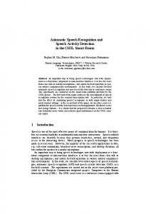
Figure 1: The convolution layer and max-pooling layer applied upon input features.

dencies with suitable context information. Using small filter sizes along the spectrogram frequency axis, the model is able to learn fine-grained localized features, while multiple stacked convolutional layers help to learn diverse features on different time/frequency scales and provide the required non-linear modeling capabilities. Unlike the time windows applied in DNN systems [2, 3, 4], the temporal modeling is deployed within convolutional layers, where we perform a 2D convolution similar to vision tasks, and multiple convolutional layers are stacked to provide a relatively large context window for each output prediction of the highest layer. The convolutional layers are followed by multiple fully connected layers and, finally, CTC is added on the top of the model. Following the suggestion from [4], we only perform pooling along the frequency band on the first convolutional layer. Specifically, we evaluate our model on phoneme recognition for the TIMIT dataset.

2.2. Activation Function The pre-activation feature maps H are passed through nonlinear activation functions. We introduce three activation functions in the following and show their functionalities in the convolutional layer as an example, notice that all the operations below are element-wise. 2.2.1. Rectifier Linear Unit Rectifier Linear Unit (ReLU) [22] is a piece-wise linear activation function that outputs zero if the input is negative and outputs the input itself otherwise. Formally, given single feature map Hi , a ReLU function is defined as follows:

2. Convolutional Neural Networks

˜ i = max(0, Hi ), H

Most of the CNN models [2, 3, 4] in the speech domain have large filters and use limited weight sharing which splits the features into limited frequency bands while performing convolution separately and the convolution is usually applied with no more than 3 layers. In this section, we describe our CNN acoustic model whose architecture is different from the above. The complete CNN includes stacked convolutional and pooling layers, at the top of which are multiple fully-connected layers. Since CNNs are adept at modeling local structures in the inputs, we use log mel-filter-bank (plus energy term) coefficients with deltas and delta-deltas which preserve the local correlations of the spectrogram.

(2)

˜ are the input and output respectively. in which H and H 2.2.2. Parametric Rectifier Linear Unit The Parametric Rectifier Linear Unit (PReLU) [23] is an extension of the ReLU in which the output of the model in the regions that input is negative is a linear function of the input with a slope of α. PReLU is formalized as:  Hi , if Hi > 0 ˜ Hi = (3) αHi , otherwise

2.1. Convolution

The extra parameter α is usually initialized to 0.1 and can be trained using backpropagation.

As shown in Figure 1, given a sequence of acoustic feature values X ∈ Rc×b×f with number of channels c, frequency bandwidth b, and time length f , the convolutional layer convolves X with k filters {Wi }k where each Wi ∈ Rc×m×n is a 3D tensor with its width along the frequency axis equal to m and its length along frame axis equal to n. The resulting k preactivation feature maps consist of a 3D tensor H ∈ Rk×bH ×fH , in which each feature map Hi is computed as follows:

Another type of activation function which has been shown to improve the results for the task of speech recognition [16, 24, 25, 26] is the maxout function [27]. Following the same computational process as in [27], we take the number of piece-wise ˜ we have: linear functions as 2 for example. Then for H

Hi = Wi ∗ X + bi , i = 1, · · · , k.

˜ i = max(Hi , Hi ), H

2.2.3. Maxout

(1)

The symbol ∗ denotes the convolution operation and bi is a bias parameter. There are three points that are worth mentioning: (1) The sequence length fH of H after convolution is guaran-

(4)

where for Hi and Hi we have: Hi = Wi ∗ X + bi , Hi = Wi ∗ X + bi ,

411

(5)

which are two linear feature map candidates after the convolution, and X is the input of the convolutional layer at Hi . Figure 2 depicts the ReLU, PReLU, and Maxout activation functions. 2.3. Pooling After the element-wise non-linearities, the features will pass through a max-pooling layer which outputs the maximum unit from p adjacent units. We do pooling only along the frequency axis since it helps to reduce spectral variations within the same speaker and between different speakers [28], while pooling in time has been shown to be less helpful [4]. Specifically, sup˜i pose that the i th feature map before and after pooling are H ˆ i , then [H ˆ i ]r,t at position (r, t) is computed by: and H ˆ i ]r,t = maxp {[H ˜ i ]r×s+j,t }, [H j=1

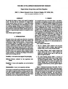
(6) Figure 3: Network structure for phoneme recognition on the TIMIT dataset. The model consists of 10 convolutional layers followed by 3 fully-connected layers on the top. All convolutional layers have the filter size of 3×5 and we use max-pooling with size of 3 × 1 only after the first convolutional layer. First and second numbers correspond to frequency and time axes respectively.

where s is the step size and p is the pooling size, and all the ˜ i ]r×s+j,t values inside the max have the same time index [H t. Consequently, the feature maps after pooling have the same sequence lengths as the ones before pooling. As shown in Figure 3, we follow the suggestions from [4] that the max pooling is performed only once after the first convolutional layer. Our intuition is that as more pooling layers are applied, units in higher layers would be less discriminative with respect to the variations in input features.

function σ: P r(Z|X) = Σo∈σ−1 (Z) P r(O|X).

3. Connectionist Temporal Classification

(8)

A dynamic programming algorithm similar to the forward algorithm for HMMs [29] is used to compute the sum in Equation 8 in an efficient way. The intermediate values of this dynamic programming can also be used to compute the gradient of ln P r(Z|X) with respect to the neural network outputs efficiently. To generate predictions from a trained model using CTC, we use the best path decoding algorithm. Since the model assumes that the latent symbols are independent given the network outputs in the framewise case, the latent sequence with the highest probability is simply obtained by emitting the most probable label at each time-step. The predicted sequence is then given by applying σ(·) to that latent sequence prediction:

Consider any sequence to sequence mapping task in which X = {X1 , ..., XT } is the input sequence and Z = {Z1 , · · · , ZL } is the target sequence. In the case of speech recognition, X is the acoustic signal and Z is a sequence of symbols. In order to train the neural acoustic model, P r(Z|X) must be maximized for each input-output pair. One way to provide a distribution over variable length output sequences given some much longer input sequence, is to introduce a many-to-one mapping of latent variable sequences O = {O1 , · · · , OT } to shorter sequences that serve as the final predictions. The probability of some sequence Z can then be defined to be the sum of the probabilities of all the latent sequences that map to that sequence. Connectionist Temporal Classification (CTC) [29] specifies a distribution over latent sequences by applying a softmax function to the output of the network for every time step, which provides a probability for emitting each label from the alphabet of output symbols at that time step P r(Ot |X). An extra blank output class ‘-’ is introduced to the alphabet for the latent sequences to represent the probability of not outputting a symbol at a particular time step. Each latent sequence sampled from this distribution can now be transformed into an output sequence using the many-to-one mapping function σ(·) which first merges the repetitions of consecutive non-blank labels to a single label and subsequently removes the blank labels as shown in Equation 7: ⎫ σ(a, b, c, −, −) ⎪ ⎪ ⎪ σ(a, b, −, c, c) ⎪ ⎪ ⎪ ⎬ σ(a, a, b, b, c) ⎪ = (a, b, c). (7) σ(−, a, −, b, c) ⎪ ⎪ ⎪ .. ⎪ ⎪ . ⎪ ⎪ ⎭ σ(−, −, a, b, c)

L ≈ σ(π ∗ ),

(9)

∗

in which π is the concatenation of the most probable output and is formalized by π ∗ = Argmaxπ P r(π|X). Note that this is not necessarily the output sequence with the highest probability. Finding this sequence is generally not tractable and requires some approximate search procedure like a beam-search.

4. Experiments In this section, we evaluate the proposed model on phoneme recognition for the TIMIT dataset. The model architecture is shown in Figure 3. 4.1. Data We evaluate our models on the TIMIT [30] corpus where we use the standard 462-speaker training set with all SA records removed. The 50-speaker development set is used for early stopping. The evaluation is performed on the core test set (including 192 sentences). The raw audio is transformed into 40dimensional log mel-filter-bank (plus energy term) coefficients with deltas and delta-deltas, which results in 123 dimensional

Therefore, the final output sequence probability is a summation over all possible sequences π that yield to Z after applying the

412

features. Each dimension is normalized to have zero mean and unit variance over the training set. We use 61 phone labels plus a blank label for training and then the output is mapped to 39 phonemes for scoring.

Table 1: Phoneme Error Rate (PER) on TIMIT. ’NP’ is the number of parameters. ’BiLSTM-3L-250H’ denotes the model has 3 bidirectional LSTM layers with 250 units in each direction. In the CNN model, (3, 5) is the filter size. Results suggest that deeper architecture and larger filter sizes leads to better performance. The best performing model on Development set, has a test PER of 18.2 %

4.2. Models Our best model consists of 10 convolutional layers and 3 fullyconnected hidden layers. Unlike the other layers, the first convolutional layer is followed by a pooling layer, which is described in section 2. The pooling size is 3 × 1, which means we only pool over the frequency axis. The filter size is 3 × 5 across the layers. The model has 128 feature maps in the first four convolutional layers and 256 feature maps in the remaining six convolutional layers. Each fully-connected layer has 1024 units. Maxout with 2 piece-wise linear functions is used as the activation function. Some other architectures are also evaluated for comparison, see section 4.4 for more details.

Model BiLSTM-3L-250H [12] BiLSTM-5L-250H [12] TRANS-3L-250H [12] CNN-(3,5)-10L-ReLU CNN-(3,5)-10L-PReLU CNN-(3,5)-6L-maxout CNN-(3,5)-8L-maxout CNN-(3,3)-10L-maxout CNN-(3,5)-10L-maxout

NP 3.8M 6.8M 4.3M 4.3M 4.3M 4.3M 4.3M 4.3M 4.3M

Dev PER 17.4% 17.2% 18.7% 17.7% 18.4% 16.7%

Test PER 18.6% 18.4% 18.3% 19.3% 18.9% 21.2% 19.8% 19.9% 18.2%

4.3. Training and Evaluation To optimize the model, we use Adam [31] with learning rate 10−4 . Stochastic gradient descent with learning rate 10−5 is then used for fine-tuning. Batch size 20 is used during training. The initial weight values were drawn uniformly from the interval [−0.05, 0.05]. Dropout [32] with a probability of 0.3 is added across the layers except for the input and output layers . L2 norm with coefficient 1e − 5 is applied at fine-tuning stage. At test time, simple best path decoding (at the CTC frame level) is used to get the predicted sequences.

datasets such as TIMIT, where over-fitting happens easily. We conjecture that the convolutional CTC model might be easier to train on phoneme-level sequences rather than the character-level. Our intuition is that the local structures within the phonemes are more robust and can easily be captured by the model. Additionally, phoneme-level training might not require the modeling of many long-term dependencies in comparison with character-level training. As a result, for a convolutional model, learning the phonemes structure seems to be easier, but empirical research needs to be done to investigate if this is indeed the case. Finally, an important point that favors convolutional over recurrent architectures is the training speed. In a CNN, the training time can be rendered virtually independent of the length of the input sequence due to the parallel nature of convolutional models and the highly optimized CNN libraries available [33]. Computations in a recurrent model are sequential and cannot be easily parallelized. The training time for RNNs increases at least linearly with the length of the input sequence.

4.4. Results Our model achieves 18.2% phoneme error rate on the core test set, which is slightly better than the LSTM baseline model and the transducer model with an explicit RNN language model. The details are presented in Table 1. Notice that the CNN model could take much less time to train in comparison with the LSTM model when keeping roughly the same number of parameters. In our setup on TIMIT, we get 2.5× faster training speed by using the CNN model without deliberately optimizing the implementation. We suppose that the gain of the computation efficiency might be more dramatic with a larger dataset. To further investigate the different structural aspects of our model, we disentangle the analysis into three sub-experiments considering the number of convolutional layers, the filter sizes and the activation functions, as shown in table 1. It turns out that the model may benefit from (1) more layers, which results in more nonlinearities and larger input receptive fields for units in the top layers; (2) reasonably large context windows, which help the model to capture the spatial/temporal relations of input sequences in reasonable time-scales; (3) the Maxout unit, which has more functional freedoms comparing to ReLU and parametric ReLU.

6. Conclusions In this work, we present a CNN-based end-to-end speech recognition framework without recurrent neural networks which are widely used in speech recognition tasks. We show promising results on the TIMIT dataset and conclude that the model has the capacity to learn the temporal relations that are required for it to be integrated with CTC. We already observed a gain in computational efficiency on the TIMIT dataset and training the model on large vocabulary datasets and integrate with the language model would be a part of our further study. Another interesting direction is to apply Batch Normalization [34] to the current model.

5. Discussion

7. Acknowledgements

Our results showed that convolutional architectures with CTC cost can achieve results comparable to the state-of-the-art by adopting the following methodology: (1) Using a significantly deeper architecture that results in a more non-linear function and also wider receptive fields along both frequency and temporal axes; (2) Using maxout non-linearities in order to make the optimization easier; and (3) Careful model regularization that yields better generalization in test time, especially for small

The experiments were conducted using Theano [35], Blocks and Fuel [36]. The authors would like to acknowledge the funding support from Samsung, NSERC, Calcul Quebec, Compute Canada, the Canada Research Chairs and CIFAR. The authors would like to thank Dmitriy Serdyuk, Dzmitry Bahdanau, Arnaud Bergeron, and Pascal Lamblin for their helpful comments.

413

8. References

[19] I. Sutskever, O. Vinyals, and Q. V. Le, “Sequence to sequence learning with neural networks,” in Advances in neural information processing systems, 2014, pp. 3104–3112.

[1] Y. LeCun, L. Bottou, Y. Bengio, and P. Haffner, “Gradient-based learning applied to document recognition,” Proceedings of the IEEE, vol. 86, no. 11, pp. 2278–2324, 1998.

[20] Q. V. Le, N. Jaitly, and G. E. Hinton, “A simple way to initialize recurrent networks of rectified linear units,” arXiv preprint arXiv:1504.00941, 2015.

[2] O. Abdel-Hamid, A.-r. Mohamed, H. Jiang, and G. Penn, “Applying convolutional neural networks concepts to hybrid NN-HMM model for speech recognition,” in Acoustics, Speech and Signal Processing (ICASSP), 2012 IEEE International Conference on. IEEE, 2012, pp. 4277–4280.

[21] W. Song and J. Cai, “End-to-End Deep Neural Network for Automatic Speech Recognition,” Technical Report. [22] X. Glorot, A. Bordes, and Y. Bengio, “Deep sparse rectifier neural networks,” in International Conference on Artificial Intelligence and Statistics, 2011, pp. 315–323.

[3] T. N. Sainath, A.-r. Mohamed, B. Kingsbury, and B. Ramabhadran, “Deep convolutional neural networks for LVCSR,” in Acoustics, Speech and Signal Processing (ICASSP), 2013 IEEE International Conference on. IEEE, 2013, pp. 8614–8618.

[23] K. He, X. Zhang, S. Ren, and J. Sun, “Delving deep into rectifiers: Surpassing human-level performance on imagenet classification,” in Proceedings of the IEEE International Conference on Computer Vision, 2015, pp. 1026–1034.

[4] T. N. Sainath, B. Kingsbury, A.-r. Mohamed, G. E. Dahl, G. Saon, H. Soltau, T. Beran, A. Y. Aravkin, and B. Ramabhadran, “Improvements to deep convolutional neural networks for LVCSR,” in Automatic Speech Recognition and Understanding (ASRU), 2013 IEEE Workshop on. IEEE, 2013, pp. 315–320.

[24] M. Cai, Y. Shi, and J. Liu, “Deep maxout neural networks for speech recognition,” in Automatic Speech Recognition and Understanding (ASRU), 2013 IEEE Workshop on. IEEE, 2013, pp. 291–296.

[5] A.-r. Mohamed, G. E. Dahl, and G. Hinton, “Acoustic modeling using deep belief networks,” Audio, Speech, and Language Processing, IEEE Transactions on, vol. 20, no. 1, pp. 14–22, 2012.

[25] X. Zhang, J. Trmal, D. Povey, and S. Khudanpur, “Improving deep neural network acoustic models using generalized maxout networks,” in Acoustics, Speech and Signal Processing (ICASSP), 2014 IEEE International Conference on. IEEE, 2014, pp. 215– 219.

[6] G. Hinton, L. Deng, D. Yu, G. E. Dahl, A.-r. Mohamed, N. Jaitly, A. Senior, V. Vanhoucke, P. Nguyen, T. N. Sainath et al., “Deep neural networks for acoustic modeling in speech recognition: The shared views of four research groups,” Signal Processing Magazine, IEEE, vol. 29, no. 6, pp. 82–97, 2012.

[26] L. T´oth, “Phone recognition with hierarchical convolutional deep maxout networks,” EURASIP Journal on Audio, Speech, and Music Processing, vol. 2015, no. 1, pp. 1–13, 2015.

[7] A. Hannun, C. Case, J. Casper, B. Catanzaro, G. Diamos, E. Elsen, R. Prenger, S. Satheesh, S. Sengupta, A. Coates et al., “Deep speech: Scaling up end-to-end speech recognition,” arXiv preprint arXiv:1412.5567, 2014.

[27] I. J. Goodfellow, D. Warde-Farley, M. Mirza, A. Courville, and Y. Bengio, “Maxout networks,” arXiv preprint arXiv:1302.4389, 2013.

[8] D. Bahdanau, J. Chorowski, D. Serdyuk, P. Brakel, and Y. Bengio, “End-to-end attention-based large vocabulary speech recognition,” arXiv preprint arXiv:1508.04395, 2015.

[28] Y. LeCun and Y. Bengio, “Convolutional networks for images, speech, and time series,” The handbook of brain theory and neural networks, vol. 3361, no. 10, p. 1995, 1995.

[9] Y. Miao, M. Gowayyed, and F. Metze, “EESEN: End-to-end speech recognition using deep RNN models and WFST-based decoding,” arXiv preprint arXiv:1507.08240, 2015.

[29] A. Graves, Supervised sequence labelling.

Springer, 2012.

[30] J. S. Garofolo, L. F. Lamel, W. M. Fisher, J. G. Fiscus, and D. S. Pallett, “DARPA TIMIT acoustic-phonetic continous speech corpus CD-ROM. NIST speech disc 1-1.1,” NASA STI/Recon Technical Report N, vol. 93, 1993.

[10] A. Graves, S. Fern´andez, F. Gomez, and J. Schmidhuber, “Connectionist temporal classification: labelling unsegmented sequence data with recurrent neural networks,” in Proceedings of the 23rd international conference on Machine learning. ACM, 2006, pp. 369–376.

[31] D. Kingma and J. Ba, “Adam: A method for stochastic optimization,” arXiv preprint arXiv:1412.6980, 2014.

[11] J. K. Chorowski, D. Bahdanau, D. Serdyuk, K. Cho, and Y. Bengio, “Attention-based models for speech recognition,” in Advances in Neural Information Processing Systems, 2015, pp. 577– 585.

[32] N. Srivastava, G. Hinton, A. Krizhevsky, I. Sutskever, and R. Salakhutdinov, “Dropout: A simple way to prevent neural networks from overfitting,” The Journal of Machine Learning Research, vol. 15, no. 1, pp. 1929–1958, 2014.

[12] A. Graves, A.-r. Mohamed, and G. Hinton, “Speech recognition with deep recurrent neural networks,” in Acoustics, Speech and Signal Processing (ICASSP), 2013 IEEE International Conference on. IEEE, 2013, pp. 6645–6649.

[33] S. Chetlur, C. Woolley, P. Vandermersch, J. Cohen, J. Tran, B. Catanzaro, and E. Shelhamer, “cudnn: Efficient primitives for deep learning,” arXiv preprint arXiv:1410.0759, 2014.

[13] A. Graves, “Sequence transduction with recurrent neural networks,” arXiv preprint arXiv:1211.3711, 2012.

[34] S. Ioffe and C. Szegedy, “Batch normalization: Accelerating deep network training by reducing internal covariate shift,” arXiv preprint arXiv:1502.03167, 2015.

[14] S. Hochreiter and J. Schmidhuber, “Long short-term memory,” Neural computation, vol. 9, no. 8, pp. 1735–1780, 1997.

[35] F. Bastien, P. Lamblin, R. Pascanu, J. Bergstra, I. Goodfellow, A. Bergeron, N. Bouchard, D. Warde-Farley, and Y. Bengio, “Theano: new features and speed improvements,” arXiv preprint arXiv:1211.5590, 2012.

[15] O. Vinyals, S. V. Ravuri, and D. Povey, “Revisiting recurrent neural networks for robust ASR,” in Acoustics, Speech and Signal Processing (ICASSP), 2012 IEEE International Conference on. IEEE, 2012, pp. 4085–4088.

[36] B. van Merri¨enboer, D. Bahdanau, V. Dumoulin, D. Serdyuk, D. Warde-Farley, J. Chorowski, and Y. Bengio, “Blocks and fuel: Frameworks for deep learning,” arXiv preprint arXiv:1506.00619, 2015.

[16] Y. Miao, F. Metze, and S. Rawat, “Deep maxout networks for lowresource speech recognition,” in Automatic Speech Recognition and Understanding (ASRU), 2013 IEEE Workshop on. IEEE, 2013, pp. 398–403. [17] S. Hochreiter, “Untersuchungen zu dynamischen neuronalen Netzen,” Master’s thesis, Institut fur Informatik, Technische Universitat, Munchen, 1991. [18] Y. Bengio, P. Simard, and P. Frasconi, “Learning long-term dependencies with gradient descent is difficult,” Neural Networks, IEEE Transactions on, vol. 5, no. 2, pp. 157–166, 1994.

414