Nov 19, 2015 - as that given class â deep network are easily fooled with ... performing open set recognition with deep networks has remained an unsolved ...... Artificial Intelligence. AAAI ..... nosis of multiple cancer types by shrunken centroids of gene expression. In Proceedings of the National Academy of Sci- ences. NAS ...
Towards Open Set Deep Networks Abhijit Bendale, Terrance E. Boult University of Colorado at Colorado Springs
arXiv:1511.06233v1 [cs.CV] 19 Nov 2015
{abendale,tboult}@vast.uccs.edu
Abstract
classification methods and large datasets have resulted in many commercial applications [5, 28, 16, 6]. However, a wide range of operational challenges occur while deploying recognition systems in the dynamic and ever-changing real world. A vast majority of recognition systems are designed for a static closed world, where the primary assumption is that all categories are known a priori. Deep networks, like many classic machine learning tools, are designed to perform closed set recognition.
Deep networks have produced significant gains for various visual recognition problems, leading to high impact academic and commercial applications. Recent work in deep networks highlighted that it is easy to generate images that humans would never classify as a particular object class, yet networks classify such images high confidence as that given class – deep network are easily fooled with images humans do not consider meaningful. The closed set nature of deep networks forces them to choose from one of the known classes leading to such artifacts. Recognition in the real world is open set, i.e. the recognition system should reject unknown/unseen classes at test time. We present a methodology to adapt deep networks for open set recognition, by introducing a new model layer, OpenMax, which estimates the probability of an input being from an unknown class. A key element of estimating the unknown probability is adapting Meta-Recognition concepts to the activation patterns in the penultimate layer of the network. OpenMax allows rejection of “fooling” and unrelated open set images presented to the system; OpenMax greatly reduces the number of obvious errors made by a deep network. We prove that the OpenMax concept provides bounded open space risk, thereby formally providing an open set recognition solution. We evaluate the resulting open set deep networks using pre-trained networks from the Caffe Model-zoo on ImageNet 2012 validation data, and thousands of fooling and open set images. The proposed OpenMax model significantly outperforms open set recognition accuracy of basic deep networks as well as deep networks with thresholding of SoftMax probabilities.
1
Recent work on open set recognition [20, 21] and open world recognition [1], has formalized processes for performing recognition in settings that require rejecting unknown objects during testing. While one can always train with an “other” class for uninteresting classes (known unknowns), it is impossible to train with all possible examples of unknown objects. Hence the need arises for designing visual recognition tools that formally account for the “unknown unknowns”[18]. Altough a range of algorithms has been developed to address this issue [4, 20, 21, 25, 2], performing open set recognition with deep networks has remained an unsolved problem. In the majority of deep networks [11, 26, 3], the output of the last fully-connected layer is fed to the SoftMax function, which produces a probability distribution over the N known class labels. While a deep network will always have a mostlikely class, one might hope that for an unknown input all classes would have low probability and that thresholding on uncertainty would reject unknown classes. Recent papers have shown how to produce “fooling” [14] or “rubbish” [8] images that are visually far from the desired class but produce high-probability/confidence scores. They strongly suggests that thresholding on uncertainty is not sufficient to determine what is unknown. In Sec. 3, we show that extending deep networks to threshold SoftMax probability improves open set recognition somewhat, but does not resolve the issue of fooling images. Nothing in the theory/practice of deep networks, even with thresholded probabilities, satisfies the formal definition of open set recognition offered in [20]. This leads to the first question addressed in this paper, “how to adapt deep networks support to open set recognition?”
Introduction
Computer Vision datasets have grown from few hundred images to millions of images and from few categories to thousands of categories, thanks to research advances in vision and learning. Recent research in deep networks has significantly improved many aspects of visual recognition [26, 3, 11]. Co-evolution of rich representations, scalable 1
MODEL Real Image Fooling OpenSet MODEL Real Image Fooling OpenSet MODEL Real Image Fooling OpenSet MODEL Real Image Fooling OpenSet
Sharks
Baseball
Baseball
Hammerhead ��
Hammerhead Shark
Real: SM 0.94 OM 0.94
Real: SM 0.57, OM 0.58
Fooling: SM 1.0, OM 0.00
Fooling: SM 0.98, OM 0.00
Openset: 0.15, OM: 0.17
Openset: SM 0.25, OM 0.10
Great White Shark
Scuba Diver
Adversarial Scuba Diver (from Hammerhead)
Whales
Dogs
Fish
Baseball
Adversarial Scuba Diver SM 0.32 Scuba Diver OM 0.49 Unknown ALer Blur OM 0.79 Hammerhead
Figure 1: Examples showing how an activation vector model provides sufficient information for our Meta-Recognition and OpenMax extension of a deep network to support open-set recognition. The OpenMax algorithm measures distance between an activation vector (AV) for an input and the model vector for the top few classes, adjusting scores and providing an estimate of probability of being unknown. The left side shows activation vectors (AV) for different images, with different AVs separated by black lines. Each input image becomes an AV, displayed as 10x450 color pixels, with the vertical being one pixel for each of 10 deep network channel activation energy and the horizontal dimension showing the response for the first 450 ImageNet classes. Ranges of various category indices (sharks, whales, dogs, fish, etc.) are identified on the bottom of the image. For each of four classes (baseball, hammerhead shark, great white shark and scuba diver), we show an AV for 4 types of images: the model, a real image, a fooling image and an open set image. The AVs show patterns of activation in which, for real images, related classes are often responding together, e.g., sharks share many visual features, hence correlated responses, with other sharks, whales, large fishes, but not with dogs or with baseballs. Visual inspection of the AVs shows significant difference between the response patterns for fooling and open set images compared to a real image or the model AV. For example, note the darker (deep blue) lines in many fooling images and different green patterns in many open set images. The bottom AV is from an “adversarial” image, wherein a hammerhead image was converted, by adding nearly invisible pixel changes, into something classified as scuba-diver. On the right are two columns showing the associated images for two of the classes. Each example shows the SoftMax (SM) and OpenMax (OM) scores for the real image, the fooling and open set image that produced the AV shown on the left. The red OM scores implies the OM algorithm classified the image as unknown, but for completeness we show the OM probability of baseball/hammerhead class for which there was originally confusion. The bottom right shows the adversarial image and its associated scores – despite the network classifying it as a scuba diver, the visual similarity to the hammerhead is clearly stronger. OpenMax rejects the adversarial image as an outlier from the scuba diver class. As an example of recovery from failure, we note that if the image is Gaussian blurred OpenMax classifies it as a hammerhead shark with .79 OM probability. The SoftMax layer is a significant component of the problem because of its closed nature. We propose an alternative, OpenMax, which extends SoftMax layer by enabling it to predict an unknown class. OpenMax incorporates likelihood of the recognition system failure. This likelihood is used to estimate the probability for a given input belonging to an unknown class. For this estimation, we adapt the concept of Meta-Recognition[22, 32, 9] to deep networks. We use the scores from the penultimate layer of deep networks (the fully connected layer before SoftMax, e.g., FC8) to estimate if the input is “far” from known training data. We call scores in that layer the activation vector(AV). This information is incorporated in our OpenMax model and used to characterize failure of recognition system. By dropping the restriction for the probability for known classes
to sum to 1, and rejecting inputs far from known inputs, OpenMax can formally handle unknown/unseen classes during operation. Our experiments demonstrate that the proposed combination of OpenMax and Meta-Recognition ideas readily address open set recognition for deep networks and reject high confidence fooling images [14]. While fooling/rubbish images are, to human observers, clearly not from a class of interest, adversarial images [8, 27] present a more difficult challenge. These adversarial images are visually indistinguishable from a training sample but are designed so that deep networks produce highconfidence but incorrect answers. This is different from standard open space risk because adversarial images are “near” a training sample in input space, for any given output class.
A key insight in our opening deep networks is noting that “open space risk” should be measured in feature space, rather than in pixel space. In prior work, open space risk is not measured in pixel space for the majority of problems [20, 21, 1]. Thus, we ask “is there a feature space, ideally a layer in the deep network, where these adversarial images are far away from training examples, i.e., a layer where unknown, fooling and adversarial images become outliers in an open set recognition problem?” In Sec. 2.1, we investigate the choice of the feature space/layer in deep networks for measuring open space risk. We show that an extreme-value meta-recognition inspired distance normalization process on the overall activation patterns of the penultimate network layer provides a rejection probability for OpenMax normalization for unknown images, fooling images and even for many adversarial images. In Fig. 1, we show examples of activation patterns for our model, input images, fooling images, adversarial images (that the system can reject) and open set images. In summary the contributions of this paper are: 1. Multi-class Meta-Recognition using Activation Vectors to estimate the probability of deep network failure 2. Formalization of open set deep networks using MetaRecognition and OpenMax, along with the proof showing that proposed approach manages open space risk for deep networks 3. Experimental analysis of the effectiveness of open set deep networks at rejecting unknown classes, fooling images and obvious errors from adversarial images, while maintaining its accuracy on testing images
2
Open Set Deep Networks
A natural approach for opening a deep network is to apply a threshold on the output probability. We consider this as rejecting uncertain predictions, rather than rejecting unknown classes. It is expected images from unknown classes will all have low probabilities, i.e., be very uncertain. This is true only for a small fraction of unknown inputs. Our experiments in Sec. 3 show that thresholding uncertain inputs helps, but is still relatively weak tool for open set recognition. Scheirer et al. [20] defined open space risk as the risk associated with labeling data that is “far” from known training samples. That work provides only a general definition and does not prescribe how to measure distance, nor does it specify the space in which such distance is to be measured. In order to adapt deep networks to handle open set recognition, we must ensure they manage/minimize their open space risk and have the ability to reject unknown inputs. Building on the concepts in [21, 1], we seek to choose a layer (feature space) in which we can build a compact abating probability model that can be thresholded to limit open space risk. We develop this model as a decaying probability
Algorithm 1 EVT Meta-Recognition Calibration for Open Set Deep Networks, with per class Weibull fit to η largest distance to mean activation vector. Returns libMR models ρj which includes parameters τi for shifting the data as well as the Weibull shape and scale parameters:κi , λi .
Require: FitHigh function from libMR Require: Activation levels in the penultimate network layer v(x) = v1 (x) . . . vN (x) Require: For each class j let Si,j = vj (xi,j ) for each correctly classified training example xi,j . 1: for j = 1 . . . N do 2: Compute mean AV, µj = meani (Si,j ) 3: EVT Fit ρj = (τj , κj , λj ) = FitHigh(kSˆj −µj k, η) 4: end for 5: Return means µj and libMR models ρj model based on distance from a learned model. In following section, we elaborate on the space and meta-recognition approach for estimating distance from known training data, followed by a methodology to incorporate such distance in decision function of deep networks. We call our methodology OpenMax, an alternative for the SoftMax function as the final layer of the network. Finally, we show that the overall model is a compact abating probability model, hence, it satisfies the definition for an open set recognition.
2.1
Multi-class Meta-Recognition
Our first step is to determine when an input is likely not from a known class, i.e., we want to add a meta-recognition algorithm [22, 32] to analyze scores and recognize when deep networks are likely incorrect in their assessment. Prior work on meta-recognition used the final system scores, analyzed their distribution based on Extreme Value Theory (EVT) and found these distributions follow Weibull distribution. Although one might use the per class scores independently and consider their distribution using EVT, that would not produce a compact abating probability because the fooling images show that the scores themselves were not from a compact space close to known input training data. Furthermore, a direct EVT fitting on the set of class post recognition scores (SoftMax layer) is not meaningful with deep networks, because the final SoftMax layer is intentionally renormalized to follow a logistic distribution. Thus, we analyze the penultimate layer, which is generally viewed as a per-class estimation. This per-class estimation is converted by SoftMax function into the final output probabilities. We take the approach that the network values from penultimate layer (hereafter the Activation Vector (AV)), are not an independent per-class score estimate, but rather they provide a distribution of what classes are “related.” In Sec. 2.2 we discuss an illustrative example based on Fig. 1. Our overall EVT meta-recognition algorithm is summarized in Alg. 1. To recognize outliers using AVs, we adapt
the concepts of Nearest Class Mean [29, 12] or Nearest Non-Outlier [1] and apply them per class within the activation vector, as a first approximation. While more complex models, such as nearest class multiple centroids (NCMC) [13] or NCM forests [17], could provide more accurate modeling, for simplicity this paper focuses on just using a single mean. Each class is represented as a point, a mean activation vector (MAV) with the mean computed over only the correctly classified training examples (line 2 of Alg. 1). Given the MAV and an input image, we measure distance between them. We could directly threshold distance, e.g., use the cross-class validation approach of [1] to determine an overall maximum distance threshold. In [1], the features were subject to metric learning to normalize them, which makes a single shared threshold viable. However, the lack of uniformity in the AV for different classes presents a greater challenge and, hence, we seek a per class metarecognition model. In particular, on line 3 of Alg. 1 we use the libMR [22] FitHigh function to do Weibull fitting on the largest of the distances between all correct positive training instances and the associated µi . This results in a parameter ρi , which is used to estimate the probability of an input being an outlier with respect to class i. Given ρi , a simple rejection model would be for the user to define a threshold that decides if an input should be rejected, e.g., ensuring 90% of all training data will have probability near zero of being rejected as an outlier. While simple to implement, it is difficult to calibrate an absolute Meta-Recognition threshold because it depends on the unknown unknowns. Therefore, we choose to use this in the OpenMax algorithm described in Sec. 2 which has a continuous adjustment. We note that our calibration process uses only correctly classified data, for which class j is rank 1. At testing, for input x assume class j has the largest probability, then ρj (x) provides the MR estimated probability that x is an outlier and should be rejected. We use one calibration for high-ranking (e.g., top 10), but as an extension separate calibration for different ranks is possible. Note when there are multiple channels per example we compute per channel per class mean vectors µj,c and Weibull parameters ρj,c . It is worth remembering that the goal is not to determine the training class of the input, rather this is a meta-recognition process used to determine if the given input is from an unknown class and hence should be rejected.
2.2
Interpretation of Activation Vectors
In this section, we present the concept of activation vectors and meta-recognition with illustrative examples based on Fig. 1. Closed Set: Presume the input is a valid input of say a hammerhead shark, i.e., the second group of activation records from Fig. 1. The activation vector shows high
scores for the AV dimension associated with a great white shark. All sharks share many direct visual features and many contextual visual features with other sharks, whales and large fish, which is why Fig. 1 shows multiple higher activations (bright yellow-green) for many ImageNet categories in those groups. We hypothesize that for most categories, there is a relatively consistent pattern of related activations. The MAV captures that distribution as a single point. The AVs present a space where we measure the distance from an input image in terms of the activation of each class; if it is a great white shark we also expect higher activations from say tiger and hammerhead sharks as well as whales, but very weak or no activations from birds or baseballs. Intuitively, this seems like the right space in which to measure the distance during training. Open Set: First let us consider an open set image, i.e., a real image from an unknown category. These will always be mapped by the deep network to the class for which SoftMax provides the maximum response, e.g., the images of rocks in Fig. 1 is mapped to baseball and the fish on the right is mapped to a hammerhead. Sometimes open set images will have lower confidence, but the maximum score will yield a corresponding class. Comparing the activation vectors of the input with the MAV for a class for which the input produced maximum response, we observe it is often far from the mean. However, for some open set images the response provided is close to the AV but still has an overall low activation level. This can occur if the input is an “unknown” class that is closely related to a known class, or if the object is small enough that it is not well distinguished. For example, if the input is from a different type of shark or large fish, it may provide a low activation, but the AV may not be different enough to be rejected. For this reason, it is still necessary for open set recognition to threshold uncertainty, in addition to directly estimating if a class is unknown. Fooling Set: Consider a fooling input image, which was artificially constructed to make a particular class (e.g., baseball or hammerhead) have high activation score and, hence, to be detected with high confidence. While the artificial construction increases the class of interest’s probability, the image generation process did not simultaneously adjust the scores of all related classes, resulting in an AV that is “far” from the model AV. Examine the 3rd element of each class group in Fig. 1 which show activations from fooling images. Many fooling images are visually quite different and so are their activation vectors. The many regions of very low activation (dark blue/purple) are likely because one can increase the output of SoftMax for a given class by reducing the activation of other classes, which in turn reduces the denominator of the SoftMax computation. Adversarial Set: Finally, consider an adversarial input image [8, 27, 31], which is constructed to be close to one class but is mislabeled as another. An example is shown
on the bottom right of Fig. 1. If the adversarial image is constructed to a nearby class, e.g., from hammerhead to great white, then the approach proposed herein will fail to detect it as a problem – fine-grained category differences are not captured in the MAV. However, adversarial images can be constructed between any pair of image classes, see [27]. When the target class is far enough, e.g., the hammerhead and scuba example here, or even farther such as hammerhead and baseball, the adversarial image will have a significant difference in activation score and hence can be rejected. We do not consider adversarial images in our experiments because the outcome would be more a function of that adversarial images we choose to generate – and we know of no meaningful distribution for that. If, for example, we choose random class pairs (a, b) and generated adversarial images from a to b, most of those would have large hierarchy distance and likely be rejected. If we choose the closest adversarial images, likely from nearby classes, the activations will be close and they will not be rejected. The result of our OpenMax process is that open set as well as fooling or adversarial images will generally be rejected. Building a fooling or adversarial image that is not rejected means not only getting a high score for the class of interest, it means maintaining the relative scores for the 999 other classes. At a minimum, the space of adversarial/fooling images is significantly reduced by these constraints. Hopefully, any input that satisfies all the constraints is an image that also gets human support for the class label, as did some of the fooling images in Figure 3 of [14], and as one sees in adversarial image pairs fine-grain separated categories such as bull and great white sharks. One may wonder if a single MAV is sufficient to represent complex objects with different aspects/views. While future work should examine more complex models that can capture different views/exemplars, e.g., NCMC [13] or NCM forests [17]. If the deep network has actually achieved the goal of view independent recognition, then the distribution of penultimate activation should be nearly view independent. While the open-jaw and side views of a shark are visually quite different, and a multi-exemplar model may be more effective in capturing the different features in different views, the open-jaws of different sharks are still quite similar, as are their side views. Hence, each view may present a relatively consistent AV, allowing a single MAV to capture both. Intuitively, while image features may vary greatly with view, the relative strength of “related classes” represented by the AV should be far more view independent.
2.3
OpenMax
The standard SoftMax function is a gradient-log-normalizer of the categorical probability distribution – a primary reason that it is commonly used as the last fully connected layer of a network. The traditional definition has per-node weights
Algorithm 2 OpenMax probability estimation with rejection of unknown or uncertain inputs.
Require: Activation vector for v(x) = v1 (x), . . . , vN (x) Require: means µj and libMR models ρj = (τi , λi , κi ) Require: α, the numer of “top” classes to revise 1: Let s(i) = argsort(vj (x)); Let ωj = 1 2: for i = 1, . . . , α do � � α−i α e
−
kx−τs(i) k λs(i)
κs(i)
ωs(i) (x) = 1 − end for 5: Revise activation vector v ˆ(x) = v(x) ◦ ω(x) P 6: Define v ˆ0 (x) = i vi (x)(1 − ωi (x)). 3: 4:
7:
v ˆj (x)
e Pˆ (y = j|x) = PN
i=0
8: 9:
evˆi (x)
(2)
Let y ∗ = argmaxj P (y = j|x) Reject input if y ∗ == 0 or P (y = y ∗ |x) < �
in their computation. The scores in the penultimate network layer of Caffe-based deep networks [10], what we call the activation vector, has the weighting performed in the convolution that produced it. Let v(x) = v1 (x), . . . , vN (x) be the activation level for each class, y = 1, . . . , N . After deep network training, an input image x yields activation vector v(x), the SoftMax layer computes: evj (x) P (y = j|x) = PN vi (x) i=1 e
(1)
where the denominator sums over all classes to ensure the probabilities over all classes sum to 1. However, in open set recognition there are unknown classes that will occur at test time and, hence, it is not appropriate to require the probabilities to sum to 1. To adapt SoftMax for open set, let ρ be a vector of metarecognition models for each class estimated by Alg. 1. In Alg. 2 we summarize the steps for OpenMax computation. For convenience we define the unknown unknown class to be at index 0. We use the Weibull CDF probability (line 3 of Alg. 2) on the distance between x and µi for the core of the rejection estimation. The model µi is computed using the images associated with category i, images that were classified correctly (top-1) during training process. We expect the EVT function of distance to provide a meaningful probability only for few top ranks. Thus in line 3 of Alg. 2, we compute weights for the α largest activation classes and use it to scale the Weibull CDF probability. We then compute revised activation vector with the top scores changed. We compute a pseudo-activation for the unknown unknown class, keeping the total activation level constant. Including the unknown unknown class, the new revised activation compute the OpenMax probabilities as in Eq. 2. OpenMax provides probabilities that support explicit rejection when the unknown unknown class (y = 0) has
ing images and 50 open set images as well as for fooling images. The more off-diagonal the more OpenMax altered the probabilities. Threshold selection for uncertainty based rejection �, would find a balance between keeping the training examples while rejecting open set examples. Fooling images were not used for threshold selection. While not part of our experimental evaluation, note that OpenMax also provides meaningful rank ordering via its estimated probability. Thus OpenMax directly supports a top-5 class output with rejection. It is also important to note that because of the re-calibration of the activation scores vˆi (x), OpenMax often does not produce the same rank ordering of the scores.
2.4 Figure 2: A plot of OpenMax probabilities vs SoftMax probabilities for the fooling (triangle), open set (square) and validation (circle) for 100 categories from ImageNet 2012. The more off-diagonal a point, the more OpenMax altered the probabilities. Below the diagonal means OpenMax estimation reduced the inputs probability of being in the class. For some inputs OpenMax increased the classes probability, which occurs when the leading class is partially rejected thereby reducing its probability and increasing a second or higher ranked class. Uncertainty-based rejection threshold (�) selection can optimize F-measure between correctly classifying the training examples while rejecting open set examples. (Fooling images are not used for threshold selection.) The number of triangles and squares below the diagonal means that uncertainty thresholding on OpenMax threshold (vertical direction), is better than thresholding on SoftMax (horizontal direction). the largest probability. This Meta-Recognition approach is a first step toward determination of unknown unknown classes and our experiments show that a single MAV works reasonably well at detecting fooling images, and is better than just thresholding on uncertainty. However, in any system that produces certainty estimates, thresholding on uncertainty is still a valid type of meta-recognition and should not be ignored. The final OpenMax approach thus also rejects unknown as well as uncertain inputs in line 9 of Alg.2. To select the hyper-parameters �, η, and α, we can do a grid search calibration procedure using a set of training images plus a sampling of open set images, optimizing Fmeasure over the set. The goal here is basic calibration for overall scale/sensitivity selection, not to optimize the threshold over the space of unknown unknowns, which cannot be done experimentally. Note that the computation of the unknown unknown class probability inherently alters all probabilities estimated. For a fixed threshold and inputs that have even a small chance of being unknown, OpenMax will reject more inputs than SoftMax. Fig. 2 shows the OpenMax and SoftMax probabilities for 100 example images, 50 train-
OpenMax Compact Abating Property
While thresholding uncertainty does provide the ability to reject some inputs, it has not been shown to formally limit open space risk for deep networks. It should be easy to see that in terms of the activation vector, the positively labeled space for SoftMax is not restricted to be near the training space, since any increase in the maximum class score increases its probability while decreasing the probability of other classes. With sufficient increase in the maximum directions, even large changes in other dimension will still provide large activation for the leading class. While in theory one might say the deep network activations are bounded, the fooling images of [14], are convincing evidence that SoftMax cannot manage open space risk. Theorem 1 (Open Set Deep Networks): A deep network extended using Meta-Recognition on activation vectors as in Alg. 2, with the SoftMax later adapted to OpenMax, as in Eq. 2, provides an open set recognition function. Proof. The Meta-Recognition probability (CDF of a Weibull) is a monotonically increasing function of kµi − xk, and hence 1 − ωi (x) is monotonically decreasing. Thus, they form the basis for a compact abating probability as defined in [21]. Since the OpenMax transformation is a weighted monotonic transformation of the MetaRecognition probability, applying Theorems 1 and 2 of [1] yield that thresholding the OpenMax probability of the unknown manages open space risk as measured in the AV feature space. Thus it is an open set recognition function.
3
Experimental Analysis
In this section, we present experiments carried out in order to evaluate the effectiveness of the proposed OpenMax approach for open set recognition tasks with deep neural networks. Our evaluation is based on ImageNet Large Scale Visual Recognition Competition (ILSVRC) 2012 dataset with 1K visual categories. The dataset contains around 1.3M images for training (with approximately 1K to 1.3K images per category), 50K images for validation and 150K
OpenMax Open set
0.60
Softmax Open set
0.59
F-measure
images for testing. Since test labels for ILSVRC 2012 are not publicly available, like others have done we report performance on validation set [11, 14, 23]. We use a pretrained AlexNet (BVLC AlexNet) deep neural network provided by the Caffe software package [10]. BVLC AlexNet is reported to obtain approximately 57.1% top-1 accuracy on ILSVRC 2012 validation set. The choice of pre-trained BVLC AlexNet is deliberate, since it is open source and one of the most widely used packages available for deep learning. To ensure proper open set evaluation, we apply a test protocol similar to the ones presented in [21, 1]. During the testing phase, we test the system with all the 1000 categories from ILSVRC 2012 validation set, fooling categories and previously unseen categories. The previously unseen categories are selected from ILSVRC 2010. It has been noted by Ruskovsky et al. [19] that approximately 360 categories from ILSVRC 2010 were discarded and not used in ILSVRC 2012. Images from these 360 categories as the open set images, i.e., unseen or unknown categories. Fooling images are generally totally unrecognizable to humans as belonging to the given category but deep networks report with near certainty they are from the specified category. We use fooling images provided by Nguyen et al. [14] that were generated by an evolutionary algorithm or by gradient ascent in pixel space. The final test set consists of 50K closed set images from ILSVRC 2012, 15K open set images (from the 360 distinct categories from ILSVRC 2010) and 15K fooling images (with 15 images each per ILSVRC 2012 categories). Training Phase: As discussed previously (Alg. 1), we consider the penultimate layer (fully connected layer 8 , i.e., FC8) for computation of mean activation vectors (MAV). The MAV vector is computed for each class by considering the training examples that deep networks training classified correctly for the respective class. MAV is computed for each crop/channel separately. Distance between each correctly classified training example and MAV for particular class is computed to obtain class specific distance distribution. For these experiments we use a distance that is a weighted combination of normalized Euclidean and cosine distances. Supplemental material shows results with pure Euclidean and other measures that overall perform similarly. Parameters of Weibull distribution are estimated on these distances. This process is repeated for each of the 1000 classes in ILSVRC 2012. The exact length of tail size for estimating parameters of Weibull distribution is obtained during parameter estimation phase over a small set of hold out data. This process is repeated multiple times to obtain an overall tail size of 20. Testing Phase: During testing, each test image goes through the OpenMax score calibration process as discussed previously in Alg. 2. The activation vectors are
0.58
0.57
0.56 0.00
0.05
0.10
0.15
0.20
0.25
Thresholds
0.30
0.35
0.40
0.45
Figure 3: OpenMax and SoftMax-w/threshold performance shown as F-measure as a function of threshold on output probabilities. The test uses 80,000 images, with 50,000 validation images from ILSVRC 2012, 15,000 fooling images and 15,000 “unknown” images draw from ILSVRC 2010 categories not used in 2012. The base deep network performance would be the same as threshold 0 of SoftMax-w/threshold. OpenMax performance gain is nearly 4.3% improvement accuracy over SoftMax with optimal threshold, and 12.3% over the base deep network. Putting that in context, over the test set OpenMax correctly classified 3450 more images than SoftMax and 9847 more than the base deep network.
the values in the FC8 layer for a test image that consists of 1000x10 dimensional values corresponding to each class and each channel. For each channel in each class, the input is compared using a per class MAV and per class Weibull parameters. During testing, distance with respect to the MAV is computed and revised OpenMax activations are obtained, including the new unknown class (see lines 5&6 of Alg. 2). The OpenMax probability is computed per channel, using the revised activations (Eq. 2) yielding an output of 1001x10 probabilities. For each class, the average over the 10 channel gives the overall OpenMax probability. Finally, the class with the maximum over the 1001 probabilities is the predicted class. This maximum probability is then subject to the uncertainty threshold (line 9). In this work we focus on strict top-1 predictions. Evaluation: ILSVRC 2012 is a large scale multi-class classification problem and top-1 or top-5 accuracy is used to measure the effectiveness of a classification algorithm [19]. Multi-class classification error for a closed set system can be computed by keeping track of incorrect classifications. For open set testing the evaluation must keep track of the errors that occur due to standard multi-class classification over known categories as well as errors between known and unknown categories. As suggested in [25, 20] we use F-measure to evaluate open set performance. For open set recognition testing, F-measure is better than accuracy because it is not inflated by true negatives.
100
OpenMax Fooling Detector Softmax Fooling Detector
OpenMax Openset Detector Softmax Openset Detector
80
Accuracy
60
40
Original AV 20
0 0.0
Agama MAV Jeep MAV 0.2
0.4
Thresholds
0.6
0.8
Crop 1 AV Crop2 AV
Figure 4: The above figure shows performance of OpenMax and SoftMax as a detector for fooling images and for open set test images. F-measure is computed for varying thresholds on OpenMax and SoftMax probability values. The proposed approach of OpenMax performs very well for rejecting fooling images during prediction phase.
For a given threshold on OpenMax/SoftMax probability values, we compute true positives, false positives and false negatives over the entire dataset. For example, when testing the system with images from validation set, fooling set and open set (see Fig. 3), true positives are defined as the correct classifications on the validation set, false positives are incorrect classifications on the validation set and false negatives are images from the fooling set and open set categories that the system incorrectly classified as known examples. Fig. 3 shows performance of OpenMax and SoftMax for varying thresholds. Our experiments show that the proposed approach of OpenMax consistently obtains higher F-measure on open set testing.
4
Discussion
We have seen that with our OpenMax architecture, we can automatically reject many unknown open set and fooling images as well as rejecting some adversarial images, while having only modest impact to the true classification rate. One of the obvious questions when using Meta-Recognition is “what do we do with rejected inputs?” While that is best left up to the operational system designer, there are multiple possibilities. OpenMax can be treated as a novelty detector in the scenario presented open world recognition [1] after that human label the data and the system incrementally learn new categories. Or detection can used as a flag to bring in other modalities[24, 7]. A second approach, especially helpful with adversarial or noisy images, is to try to remove small noise that might have lead to the miss classification. For example, the bottom right of Fig. 1, showed an adversarial image wherein a hammerhead shark image with noise was incorrectly classified by base deep network as a scuba diver. OpenMax
Lizards
Jeep
Figure 5: OpenMax also predict failure during training as in this example. The official class is agama but the MAV for agama is rejected for this input, and the highest scoring class is jeep with probability 0.26. However, cropping out image regions can find windows where the agama is well detected and another where the Jeep is detected. Crop 1 is the jeep region, crop 2 is agama and the crops AV clearly match the appropriate model and are accepted with probability 0.32 and 0.21 respectively.
Rejects the input, but with a small amount of simple gaussian blur, the image can be reprocessed and is accepted as a hammerhead shark by with probability 0.79. We used non-test data for parameter tuning, and for brevity only showed performance variation with respect to the uncertainty threshold shared by both SoftMax with threshold and OpenMax. The supplemental material shows variation of a wider range of OpenMax parameters, e.g. one can increase open set and fooling rejection capability at the expense of rejecting more of the true classes. In future work, such increase in true class rejection might be mitigated by increasing the expressiveness of the AV model, e.g. moving to multiple MAVs per class. This might allow it to better capture different contexts for the same object, e.g. a baseball on a desk has a different context, hence, may have different “related” classes in the AV than say a baseball being thrown by a pitcher. Interestingly, we have observe that the OpenMax rejection process often identifies/rejects the ImageNet images that the deep network incorrectly classified, especially images with multiple objects. Similarly, many samples that are far away from training data have multiple objects in the scene. Thus, other uses of the OpenMax rejection can be to improve training process and aid in developing better localization techniques [30, 15]. See Fig. 5 for an example.
5
Towards Open Set Deep Networks: Supplemental
In this supplement, we provide we provide additional material to further the readers understanding of the work on Open Set Deep Networks, Mean Activation Vectors, Open Set Recognition and OpenMax algorithm. We present additional experiments on ILSVRC 2012 dataset. First we present experiments to illustrate performance of OpenMax for various parameters of EVT calibration (alg. 1, main paper) followed by sensitivity of OpenMax to total number of “top classes” (i.e. α in alg. 2, main paper) to consider for recalibrating SoftMax scores. We then present different distance measures namely euclidean and cosine distance used for EVT calibration. We then illustrate working of OpenMax with qualitative examples for open set evaluation performed during the testing phase. Finally, we illustrate the distribution of Mean Activation Vectors with a class confusion map.
6 6.1
Parameters for OpenMax Calibration Tail Sizes for EVT Calibration
In this section we present extended analysis of effect of tail sizes used for EVT fitting in Alg 1 in main paper on the performance of the proposed OpenMax algorithm. We tried multiple tail sizes for estimating parameters of Weibull distribution (line 3, Alg 1, main paper). We found that as the tail size increased, OpenMax algorithm became very robust at rejecting images from open set and fooling set. OpenMax continued to perform much better than SoftMax in this setting. The results of this experiments are presented in Fig 6. However, beyond tail size 20, we saw performance drop on validation set. This phenomenon can be seen in Fig 7, since F-Measure obtained on OpenMax starts to drop beyond tail size 20. Thus, there is an optimal balance to be maintained between rejecting images from open set and fooling set, while maintaining correct classification rate on validation set of ILSVRC 2012.
6.2
Top Classes to be considered for revision α
In Alg 2 of the main paper, we present a methodology to calibrate FC8 scores via OpenMax. In this process, we also incorporate a process to adjust class probability as well as estimating the probability for the unknown unknown class. For this purpose, in Alg 2 (main paper), we consider “top” classes to revise (line 2, Alg 2, main paper), which is controlled by parameter α. We call this parameter as α rank, where value of α suggests total number of “top” classes to revise. In our experiments we found that optimal performance is obtained when α = 10. At lower values of α we see drop in F-Measure performance. If we continue
to increase α values beyond 10, we see almost no gain in F-Measure performance or fooling/open set detection accuracy. The most likely reason for this lack of change in performance beyond α = 10 is lower ranked classes have very small FC8 activations and do not provide any significant change in OpenMax probability. The results for varying values of α are presented in Figs 8 and 9.
6.3
Distance Measures
We tried different distance measures to compute distances between Mean Activation Vectors and Activation Vector of an incoming test image. We tried cosine distance, euclidean distance and euclidean-cosine distance. Cosine distance and euclidean distances compared marginally worse compared to euclidean-cosine distance. Cosine distance does not provide for a compact abating property hence may not restrict open space for points that have small degree of separation in terms of angle but still far away in terms of euclidean distance. Euclidean-cosine distance finds the closest points in a hyper-cone, thus restricting open space and finding closest points to Mean Activation Vector. Euclidean distance and euclidean-cosine distance performed very similar in terms of performance. In Fig 10 we show effect of different distances on over all performance. We see that OpenMax still performs better than SoftMax, and euclidean-cosine distance performs the best of those tested.
7
Qualitative Examples
It is often useful to look at qualitative examples of success and failure. Fig. 11 – Fig. 12 shows examples where OpenMax failed to detect open set examples. Some of these were from classess in ILSVRC 2010 that were close but not identical to classes in ILSVRC 2012. Other examples are objects from distinct ILSVRC 2010 classes that were visually very similar to a particular object class in ILSVRC 2012. Finally we show an example where OpenMax processed a ILSVRC 2012 validation image but reduced its probability thus Caffe with SoftMax provides the correct answer but OpenMax gets this example wrong.
8
Confusion Map of Mean Activation Vectors
Because detection/rejection of unknown classes depends on the distance mean activation vector (MAV) of the highest scoring FC8 classes. Note this is different from finding the distance from the input to the cloest MAV. However, we still find that for unknown classes that are only fine-grain variants of known classes, the system will not likely reject them. Similarly for adversarial images, if an image is adversarially modified to a “neary-by” is is much less likely the OpenMax will reject/detect it. Thus it is useful to consider the confusion between existing classes.
OpenMax Fooling Detector Softmax Fooling Detector
OpenMax Openset Detector Softmax Openset Detector
OpenMax Openset Detector Softmax Openset Detector
80
70
70
70
60
60
60
50 40
50 40
30
30
30
20
20
20
0 0.00
10 0.05
0.10
0.15
0.20
0.25
Thresholds
0.30
0.35
0.40
0 0.00
0.45
(a) Tail Size 10
OpenMax Fooling Detector Softmax Fooling Detector
90
10 0.05
0.10
0.15
0.20
0.25
Thresholds
0.30
0.35
0.40
0 0.00
0.45
OpenMax Fooling Detector Softmax Fooling Detector
90
OpenMax Openset Detector Softmax Openset Detector
80 70
70
60
60
60
50 40 30
30
20
20
10 0.15
0.20
0.25
Thresholds
0.30
(d) Tail Size 30
0.35
0.40
0.45
0 0.00
0.30
0.35
0.40
0.45
OpenMax Openset Detector Softmax Openset Detector
50
30
0.10
0.25
Thresholds
40
20 10
0.20
80
Accuracy
Accuracy
50 40
0.15
OpenMax Fooling Detector Softmax Fooling Detector
90
70
0.05
0.10
(c) Tail Size 25
80
0 0.00
0.05
(b) Tail Size 20 (optimal)
OpenMax Openset Detector Softmax Openset Detector
OpenMax Openset Detector Softmax Openset Detector
80
Accuracy
50 40
OpenMax Fooling Detector Softmax Fooling Detector
90
80
10
Accuracy
OpenMax Fooling Detector Softmax Fooling Detector
90
Accuracy
Accuracy
90
10 0.05
0.10
0.15
0.20
0.25
Thresholds
0.30
(e) Tail Size 40
0.35
0.40
0.45
0 0.00
0.05
0.10
0.15
0.20
0.25
Thresholds
0.30
0.35
0.40
0.45
(f) Tail Size 50
Figure 6: The graphs shows fooling detection accuracy and open set detection accuracy for varying tail sizes of EVT fitting. The graphs plot accuracy vs varying uncertainty threshold values, with different tails in each graph. We observe that OpenMax consistently performs better than SoftMax for varying tail sizes. However, while increasing tail size increases OpenMax rejections for open set and fooling, it also increases rejection for true images thereby reducing accuracy on validation set as well, see Fig 7. These type of accuracy plots are often problematic for open set testing which is why in Fig 7 we use F-measure to better balance rejection and true acceptance. In the main paper, tail size of 20 was used for all the experiments.
9
Comparison with the 1-vs-set algorithm.
The main paper focused on direct extensions within the Deep Networks. While we consider it tangential, reviewers might worry that applying other models, e.g. a linear based 1-vs-set open set algorithm[20] to the FC8 data would provide better results. For completeness we did run these experiments. We used liblinear to train a linear SVM on the training samples from the 1000 classes. We also trained a 1-vs-set machine using the liblinear extension cited in [1], refining it on the training data for the 1000 classes. The 1-Vs-Set algorithm achieves an overall F-measure of only .407, which is much lower than the .595 of the OpenMax approach.
References [1] A. Bendale and T. E. Boult. Towards open world recognition. In The IEEE Conference on Computer Vision and Pattern Recognition (CVPR), pages 1893–1902, June 2015. 1, 3, 4, 6, 7, 8, 10
[2] P. Bodesheim, A. Freytag, E. Rodner, and J. Denzler. Local novelty detection in multi-class recognition problems. In Winter Conference on Applications of Computer Vision, 2015 IEEE Conference on. IEEE, 2015. 1 [3] K. Chatfield, K. Simonyan, A. Vedaldi, and A. Zisserman. Return of the devil in the details: Delving deep into convolutional nets. In Proceedings of the British Machine Vision Conference,(BMVC), 2014. 1 [4] Q. Da, Y. Yu, and Z.-H. Zhou. Learning with augmented class by exploiting unlabeled data. In AAAI Conference on Artificial Intelligence. AAAI, 2014. 1 [5] T. Dean, M. A. Ruzon, M. Segal, J. Shlens, S. Vijayanarasimhan, and J. Yagnik. Fast, accurate detection of 100,000 object classes on a single machine. In Computer Vision and Pattern Recognition (CVPR), 2013 IEEE Conference on, pages 1814–1821. IEEE, 2013. 1 [6] H. Fang, S. Gupta, F. Iandola, R. Srivastava, L. Deng, P. Dollar, J. Gao, X. He, M. Mitchell, P. John, L. Zitnick, and G. Zweig. From captions to visual concepts and back. In The IEEE Conference on Computer Vision and Pattern Recognition (CVPR). IEEE, 2015. 1 [7] A. Frome, G. S. Corrado, J. Shlens, S. Bengio, J. Dean, T. Mikolov, et al. Devise: A deep visual-semantic embed-
OpenMax Fooling Detector
Softmax Fooling Detector
OpenMax Fooling Detector
OpenMax Fooling Detector
0.59
0.59
0.59
0.58
0.58
0.57
F-measure
0.57 0.56
0.56
0.57 0.56
0.55
0.55
0.55
0.54
0.54
0.54
0.05
0.10
0.15
0.20
0.25
Thresholds
0.30
0.35
0.40
0.53 0.00
0.45
(a) Tail Size 10
OpenMax Fooling Detector
0.05
0.10
0.15
0.20
0.25
0.30
Thresholds
0.35
0.40
0.53 0.00
0.45
Softmax Fooling Detector
OpenMax Fooling Detector
Softmax Fooling Detector
0.59
0.59
0.58
0.58
0.58
0.57
0.57
0.57
F-measure
0.59
F-measure
0.60
0.55
0.56 0.55
0.54
0.15
0.20
0.25
0.30
Thresholds
0.35
0.40
0.53 0.00
0.45
0.20
0.25
0.30
Thresholds
0.35
0.40
0.45
Softmax Fooling Detector
0.56 0.55
0.54
0.10
0.15
OpenMax Fooling Detector
0.60
0.05
0.10
(c) Tail Size 25
0.60
0.53 0.00
0.05
(b) Tail Size 20 (optimal)
0.56
Softmax Fooling Detector
0.60
0.58
0.53 0.00
F-measure
Softmax Fooling Detector
0.60
F-measure
F-measure
0.60
0.54
0.05
0.10
(d) Tail Size 30
0.15
0.20
0.25
Thresholds
0.30
0.35
0.40
0.53 0.00
0.45
0.05
0.10
(e) Tail Size 40
0.15
0.20
0.25
Thresholds
0.30
0.35
0.40
0.45
(f) Tail Size 50
Figure 7: The graphs shows F-Measure performance of OpenMax and Softmax with Open Set testing (using validation, fooling and open set images for testing). Each graph shows F-measure plotted against varying uncertainty threshold values. Tail size varies in different plots. OpenMax reaches its optimal performance at tail size 20. For tail sizes larger than 20, though OpenMax becomes good at rejecting images from fooling set and open set (Fig 6), it also rejects true images thus reducing accuracy on validation set. Hence, we choose tail size 20 for our experiments in main paper. OpenMax Fooling Detector
Softmax Fooling Detector
OpenMax Fooling Detector
Softmax Fooling Detector
0.60
0.59
0.59
0.58
0.58
0.57
0.57
F-measure
F-measure
0.60
0.56
0.56
0.55
0.55
0.54
0.54
0.53 0.00
0.05
0.10
0.15
0.20
0.25
Thresholds
0.30
0.35
0.40
0.45
(a) Tail Size 20, Alpha Rank 5
0.53 0.00
0.05
0.10
0.15
0.20
0.25
Thresholds
0.30
0.35
0.40
0.45
(b) Tail Size 20, Alpha Rank 10 (optimal)
Figure 8: The above figure shows performance of OpenMax and Softmax as number of top classes to be considered for recalibrating are changed. In our experiments, we found best performance when top 10 classes (i.e. α = 10) were considered for recalibration. ding model. In Advances in Neural Information Processing Systems, pages 2121–2129, 2013. 8 [8] I. Goodfellow, J. Shelns, and C. Szegedy. Explaining and harnessing adversarial examples. In International Conference on Learning Representations. Computational and Bio-
logical Learning Society, 2015. 1, 2, 4 [9] N. Jammalamadaka, A. Zisserman, M. Eichner, V. Ferrari, and C. Jawahar. Has my algorithm succeeded? an evaluator for human pose estimators. In Computer Vision–ECCV 2012. Springer, 2014. 2
OpenMax Fooling Detector Softmax Fooling Detector
90
OpenMax Openset Detector Softmax Openset Detector
80
OpenMax Openset Detector Softmax Openset Detector
80
70
70
60
60
50
Accuracy
F-measure
OpenMax Fooling Detector Softmax Fooling Detector
90
40
50 40
30
30
20
20
10
10
0 0.00
0.05
0.10
0.15
0.20
0.25
Thresholds
0.30
0.35
0.40
0 0.00
0.45
(a) Tail Size 20, Alpha Rank 5
0.05
0.10
0.15
0.20
0.25
Thresholds
0.30
0.35
0.40
0.45
(b) Tail Size 20, Alpha Rank 10 (optimal)
Figure 9: The figure shows fooling detection and open set detection accuracy for varying alpha sizes. In our experiments, alpha rank of 10 yielded best results. Increasing alpha value beyond 10 did not result in any performance gains. OpenMax Fooling Detector
Softmax Fooling Detector
0.60
OpenMax Open set
Softmax Open set
OpenMax Open set
0.59
0.59
0.59 0.58
0.58
0.57
0.56
F-measure
0.58
F-measure
F-measure
Softmax Open set
0.57
0.57 0.56 0.55
0.56 0.54 0.55 0.53 0.00
0.55 0.54 0.00
0.05
0.10
0.15
0.20
0.25
Thresholds
0.30
0.35
0.40
0.45
0.00
0.05
0.10
0.15
0.20
0.25
Thresholds
0.30
0.35
0.40
0.05
0.10
0.15
0.20
0.25
Thresholds
0.30
0.35
0.40
0.45
0.45
(c) Euclidean-Cosine distance, Tail Size (a) Cosine Distance, Tail Size 20, Alpha (b) Euclidean Distance, Tail Size 20, 20, Alpha Rank 10 (optimal) Note scale difference! Rank 10 Alpha Rank 10
Figure 10: The above figure shows performance of OpenMax and Softmax for different types of distance measures. We found the performance trend to be similar, with euclidean-cosine distance performing best. [10] Y. Jia, E. Shelhamer, J. Donahue, S. Karayev, J. Long, R. Girshick, S. Guadarrama, and T. Darrell. Caffe: Convolutional architecture for fast feature embedding. arXiv preprint arXiv:1408.5093, 2014. 5, 7 [11] A. Krizhevsky, I. Sutskever, and G. E. Hinton. Imagenet classification with deep convolutional neural networks. In Advances in neural information processing systems (NIPS), pages 1097–1105, 2012. 1, 7 [12] T. Mensink, J. Verbeek, F. Perronnin, and G. Csurka. Metric learning for large scale image classification: Generalizing to new classes at near-zero cost. In ECCV, 2012. 3 [13] T. Mensink, J. Verbeek, F. Perronnin, and G. Csurka. Distance-based image classification: Generalizing to new classes at near-zero cost. Pattern Analysis and Machine Intelligence, IEEE Transactions on, 35(11):2624–2637, 2013. 4, 5 [14] A. Nguyen, J. Yosinski, and J. Clune. Deep neural networks are easily fooled: High confidence predictions for unrecognizable images. In Computer Vision and Pattern Recognition (CVPR), 2015 IEEE Conference on. IEEE, 2015. 1, 2, 5, 6, 7
[15] M. Oquab, L. Bottou, I. Laptev, and J. Sivic. Is object localization for free? weakly-supervised learning with convolutional neural networks. In The IEEE Conference on Computer Vision and Pattern Recognition (CVPR), June 2015. 8 [16] V. Ordonez, V. Jagadeesh, W. Di, A. Bhardwaj, and R. Piramuthu. Furniture-geek: Understanding fine-grained furniture attributes from freely associated text and tags. In Applications of Computer Vision (WACV), 2014 IEEE Winter Conference on, pages 317–324. IEEE, 2014. 1 [17] M. Ristin, M. Guillaumin, J. Gall, and L. VanGool. Incremental learning of ncm forests for large scale image classification. CVPR, 2014. 4, 5 [18] D. Rumsfeld. Known and unknown: a memoir. Penguin, 2011. 1 [19] O. Russakovsky, J. Deng, H. Su, J. Krause, S. Satheesh, S. Ma, Z. Huang, A. Karpathy, A. Khosla, M. Bernstein, A. C. Berg, and L. Fei-Fei. ImageNet Large Scale Visual Recognition Challenge. International Journal of Computer Vision (IJCV), pages 1–42, April 2015. 7 [20] W. J. Scheirer, A. de Rezende Rocha, A. Sapkota, and T. E. Boult. Toward open set recognition. Pattern Analysis and
Figure 11: Left is an Image from ILSVRC 2010, “subway train”, n04349306. OpenMax and Softmax both classify as n04335435. Instead of ‘unknown”. OpenMax predicts that the image on left belongs to category “n04335435:streetcar, tram, tramcar, trolley, trolley car” from ILSVRC 2012 with an output probability of 0.6391 (caffe probability 0.5225). Right is an example image image from ILSVRC 2012, “streetcar, tram, tramcar, trolley, trolley car”, n04335435 It is easy to see such mistakes are bound to happen since open set classes from ILSVRC 2010 may have have many related categories which have different names, but which are semantically or visually are very similar. This is why fooling rejection is much stronger than open set rejection.
(a) A validation example of Openmax Failure/ Softmax labeles it correctly as n03977966 (Police van/police wagon) with probability 0.6463, while openmax incorrect labels it n02701002 (Ambulance) with probability 0.4507. )
(b) Another validation failure example, where softmax classifies it as n13037406 with probability 0.9991, while OpenMax rejects it as unknown. n13037406 is a gyromitra, which is genus of mushroom.
Figure 12: The above figure shows an examples of validation image misclassification by OpenMax algorithm. Machine Intelligence, IEEE Transactions on, 35(7):1757– 1772, 2013. 1, 3, 7, 10 [21] W. J. Scheirer, L. P. Jain, and T. E. Boult. Probability models for open set recognition. Pattern Analysis and Machine Intelligence, IEEE Transactions on, 36(11):2317–2324, 2014. 1, 3, 6, 7 [22] W. J. Scheirer, A. Rocha, R. J. Micheals, and T. E. Boult. Meta-recognition: The theory and practice of recognition score analysis. Pattern Analysis and Machine Intelligence, IEEE Transactions on, 33(8):1689–1695, 2011. libMR code at http://metarecognition.com. 2, 3, 4
[23] K. Simonyan and A. Zisserman. Very deep convolutional networks for large scale image recognition. In International Conference on Learning Representations. Computational and Biological Learning Society, 2015. 7 [24] R. Socher, M. Ganjoo, C. D. Manning, and A. Ng. Zero-shot learning through cross-modal transfer. In Advances in neural information processing systems, pages 935–943, 2013. 8 [25] R. Socher, C. D. Manning, and A. Y. Ng. Learning continuous phrase representations and syntactic parsing with recursive neural networks. In Proceedings of the NIPS-2010 Deep Learning and Unsupervised Feature Learning Work-
Figure 13: The above figure shows confusion matrix of distances between Mean Activation Vector (MAV) for each class in ILSVRC 2012 with MAV of every other class. Lower values of distances indicate that MAVs for respective classes are very close to each other, and higher values of distances indicate classes that are far apart. Majority of misclassifications for OpenMax happen in fine-grained categorization, which is to be expected. shop, pages 1–9, 2010. 1, 7 [26] C. Szegedy, W. Liu, Y. Jia, P. Sermanet, S. Reed, D. Anguelov, D. Erhan, V. Vanhoucke, and A. Rabinovich. Going deeper with convolutions. In Computer Vision and Pattern Recognition (CVPR), 2015 IEEE Conference on. IEEE, 2015. 1 [27] C. Szegedy, W. Zaremba, I. Sutskever, J. Bruna, D. Erhan, I. Goodfellow, and R. Fergus. Intriguing properties of neural networks. In International Conference on Learning Representations. Computational and Biological Learning Society, 2014. 2, 4, 5 [28] Y. Taigman, M. Yang, M. Ranzato, and L. Wolf. Deepface: Closing the gap to human-level performance in face verification. In Computer Vision and Pattern Recognition (CVPR), 2014 IEEE Conference on, pages 1701–1708. IEEE, 2014. 1
[29] R. Tibshirani, T. Hastie, B. Narasimhan, and G. Chu. Diagnosis of multiple cancer types by shrunken centroids of gene expression. In Proceedings of the National Academy of Sciences. NAS, 2002. 3 [30] A. Vezhnevets and V. Ferrari. Object localization in imagenet by looking out of the window. In Proceedings of the British Machine Vision Conference,(BMVC), 2015. 8 [31] J. Yosinski, J. Clune, A. Nguyen, T. Fuchs, and H. Lipson. Understanding neural networks through deep visualization. In International Conference on Machine Learning, Workshop on Deep Learning, 2015. 4 [32] P. Zhang, J. Wang, A. Farhadi, M. Hebert, and D. Parikh. Predicting failures of vision systems. In The IEEE Conference on Computer Vision and Pattern Recognition (CVPR), June 2014. 2, 3