Towards Real-Time Traffic Sign Recognition by Class ... - CiteSeerX

Towards Real-Time Traffic Sign Recognition by Class-Specific Discriminative Features Andrzej Ruta Yongmin Li Xiaohui Liu School of Information Systems, Computing and Mathematics Brunel University, Uxbridge, Middlesex UB8 3PH, UK {Andrzej.Ruta, Yongmin.Li, Xiaohui.Liu}@brunel.ac.uk Abstract

Real-time road sign recognition has been of great interest for many years. This problem is often addressed in a two-stage procedure involving detection and classification. In this paper a novel approach to sign representation and classification is proposed. In many previous studies focus was put on deriving a set of discriminative features from a large amount of training data using global feature selection techniques e.g. Principal Component Analysis or AdaBoost. In our method we have chosen a simple yet robust image representation built on top of the Colour Distance Transform (CDT). Based on this representation, we introduce a feature selection algorithm which captures a variable-size set of local image regions ensuring maximum dissimilarity between each individual sign and all other signs. Experiments have shown that the discriminative local features extracted from the template sign images enable minimum-distance classification with error rate not exceeding 7%.

1 Introduction Recognition of traffic signs has been a challenge problem for many years and is an important task for the intelligent vehicles. Although the first work in this area can be traced back to the late 1960’s, only in the 1990’s, when the problems of intelligent navigation and driver’s safety attracted worldwide attention, significant advances were made. Nevertheless, there is still an apparent gap between what human and machine can do, making the attentive driver an irreplaceable guarantor of safety in the traffic environment. Road signs have unique properties distinguishing them from the multitude of other outdoor objects. These properties were benefited from in numerous attempts to build an efficient detection and recognition system. In the majority of published work a twostage sequential approach was adopted, aiming at locating the regions of interest first, and subsequently passing them to the classifier [1, 2, 3]. To detect possible sign candidates traditionally colour information is extracted [1, 2], followed by the geometrical edge [1, 4] or corner analysis [2]. Alternative approaches utilise distance transform [5] or neural networks [6]. In several studies the geometrical tracking aspect was given consideration [1, 6, 7]. However, reliable prediction of the geometrical properties of signs from a moving vehicle is complex in general as the vehicle’s manoeuvres are enforced by the

actual traffic situation and therefore cannot be apriori known. To overcome this problem, the above approaches impose simplified motion model, e.g. assuming constant velocity. In the classification stage a pixel-based approach is often adopted and the class of the detected sign is determined by the cross-correlation template matching [1] or neural network [2]. Feature-based approach is used for instance in [3]. More recently, Bahlmann et al. [9] adopted the ideas of Viola and Jones [8] to detect traffic signs based on the colour-sensitive Haar wavelet features and AdaBoost framework. In the classification stage, assuming Gaussian class distribution and the independence of consecutive frame observations, Bayes classifier is used to fuse the individual observations over time. Only 6% error rate is reported using this method. Pacl´ık et al. [10] introduced a different strategy built upon the claim that a candidate sign can be represented as a set of similarities to the stored prototype images. For each class similarity assessment is made with respect to a different set of local regions refined in the training process. In this work we have developed a two-stage road sign detection and classification system. Figure 1 shows an example frame from video input with a road sign detected and recognised. More specifically, our detector is a form of well-constrained circle/regular polygon detector introduced in [4], augmented with the appropriate colour pre-filtering. In the classification stage, motivated by [10], we introduce a novel feature selection algorithm built on top of the Colour Distance Transform (CDT) image representation. We show that although our algorithm generates sign descriptors of variable dimensionality, individual classification scores can be made directly comparable due to the global selection criterion used. In consequence the proposed method seems to be a more natural way of discrimination among signs, as not the same amount of information is necessary to tell different classes apart. The rest of this paper is organised as follows: In section 2 traffic sign detection and tracking are briefly described. Sections 3 and 4 discuss the main contributions of this work, discriminative feature selection and sign classification. Section 5 presents experimental results on the real traffic video sequences. Finally, conclusions are Figure 1: Screenshot from our traffic sign recognition system in action. drawn in section 6.

2 Sign Detection and Tracking Our road sign detector is triggered every fixed number of frames to capture new candidates emerging in the scene. It makes use of the apriori knowledge about the model signs, uniquely identified by their general shape, colour and contained ideogram. Based on the first two properties four sign categories coinciding with the well-known semantic families are identified: instruction (blue circular), prohibitive (red circular), cautionary (yellow triangular), and informative (blue square) signs. As we believe the shape and boundary colour of a sign are sufficient visual cues to locate the candidates reliably, the proposed

detector operates on the colour gradient and edge maps of the original video frames. Furthermore, it uses a generalisation of Hough Transform introduced in [4], which is motivated by the fact that the targeted objects are all instances of equiangular polygons, including circles that can be though of as such polygons with the infinite number of sides. Original regular polygon transform is augmented with the appropriate image preprocessing intended to enhance edges of specific colour. For each RGB pixel~x = [xR , xG , xB ] and s = xR + xG + xB a simple colour enhancement is provided by a set of transformations: fR (~x) = max(0, min((xR − xG )/s, (xR − xB )/s)) fB (~x) = max(0, min((xB − xR )/s, (xB − xG )/s)) . fY (~x) = max(0, min((xR − xB )/s, (xG − xB )/s))

(1)

Transforms defined in (1) effectively extract the red, blue, and yellow image fragments. In the resulting images colour-specific edge maps are extracted by a simple filter which for a given pixel picks the highest difference among the pairs of neighbouring pixels that could be used to form a straight line through the middle pixel being tested. Obtained values are further thresholded and only in the resulting edge pixels values of directional and magnitude gradient are calculated. This technique is adequate to our problem as it enables a quick extraction of edges and avoids expensive computation of the whole gradient magnitude map which, with the exception of the sparse edge pixels, is of no use to the shape detector. For a given pair of gradient and edge images associated with colour c, appropriate instances of the Loy & Barnes’s detector are run to yield a set of possible sign shapes. For instance, for a “blue pair” a circular shape detector is triggered to search for the blue instruction signs, e.g. “turn left” or “turn right”, and a square detector is run to detect potential square information signs, e.g. “pedestrian crossing” or “parking place”. As each found candidate has known shape and border colour c, detector serves as a pre-classifier reducing the number of possible templates to analyse in the later stage to the ones contained in either category. When signs are in the cluttered background, a number of false candidates may be produced. To address this issue, an additional step is taken to verify the presence of colours appropriate for the just found category. Once a candidate sign is detected, it is unnecessary to seek it in the consecutive frames in every possible location. Assuming motion with constant velocity along the optical axis of the camera, we have employed a Kalman filter [11] to track a sign detected in a previous frame of an input video. The state of the tracker is defined by (x, y, s), where x, y are coordinates of the sign’s centre in the image, and s is the scale factor to the standard sign templates. In the current implementation we use the mean and variance estimates from the Kalman filter to locate the centre and the size of the local search region in the next video frame. Therefore, computation has been significantly reduced compared to the exhaustive search over the whole image.

3 Image Representation and Feature Selection Selecting an optimal feature set for a large number of template images is a non-trivial task. We have experimented with several techniques such as Principal Component Analysis and AdaBoost. Aiming at retrieving the global variance of a whole data set, PCA is not capable of capturing features critical to the individual templates. AdaBoost on the other hand, although generating efficient classifiers, is not entirely convincing in terms of the fixed cardinality of the feature set being extracted. Clearly, certain signs are very dis-

tinctive and analysis of only a few small regions suffice to distinguish them even among tens of others. Meanwhile, there are groups of very similar signs that look tightly clustered, even in a highly multidimensional feature space. This complex nature of similarity between templates raises a question whether there is sufficient justification for classifying the signs based on the same set of features. Motivated by [10], we propose here an algorithm that relaxes the above limitation by extracting for each model sign a limited number of local image regions in which it looks possibly the most different from all other templates residing in the same category. The same discriminative regions are further used to compare a video frame image with the templates and make a reliable on-line classification. Below we first outline the process of converting the raw bitmap images into a more suitable discrete-colour representation. Second, we introduce the notion of local image region and dissimilarity. Finally, the implementation of the discriminative region selection algorithm is discussed.

3.1 Colour Discretisation Detected sign images come as rectangular regions containing the target object and, depending on its shape, also background fragments, as depicted in Fig. 2. In order to prepare the candidate for classification, the image is first scaled to a common size, typically 60 × 60 pixels. Undesirable background regions are then masked out using the information about the object’s shape and orientation provided by the detector [4]. It is important to note that the full colour spectrum is far more than necessary to identify the object, as the signs contain only up to four distinctive colours per category. Therefore, the candidate images are finally subject to on-line colour discretisation according to the category-specific colour models learned off-line from a set of training images as follows. For each category of signs a number of frames are picked randomly from the real video sequences depicting the respective signs. Then, the Expectation Maximisation algorithm [12] is employed to estimate an optimal Gaussian Mixture model for each colour specific to this category. The procedure is restarted several times for the increasing number of randomly initialised Gaussian components to refine the estimation. The best model in terms of the mean data likelihood is selected. To speed up the on-line segmentation, offline learned models are used by a Bayes classifier to assign the appropriate colour to each possible RGB triple, yielding a look-up table with 2553 entries for each category. Sample results of the on-line colour discretisation are illustrated in Fig. 2.

Figure 2: Sample images obtained by sign detector before (above) and after (below) background masking and colour discretisation; 2 bits suffice to encode colours in each image. Along with the observed candidate sign images also the model images are discretised. However, as they already contain ideal colours, discretisation merely aims here at collapsing the physical 24-bit bitmap representation to the 2-bit image with the specific colour indices encoded. A set of thresholds is applied to the templates in Hue-Saturation-Value space to complete this task. Furthermore, for each discrete colour present in the resulting

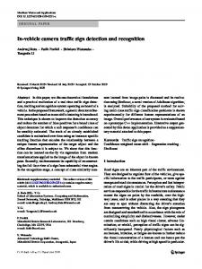
images a separate distance transform [13] is computed, giving output similar to this shown in Fig. 3. In DT computation pixels of a given colour are simply treated as feature pixels and all the remaining ones as non-feature pixels. (3, 4) Chamfer metric [14] is used to approximate Euclidean distance between the feature pixels. To emphasise a strong relation to colour, we call this variant of DT a Colour Distance Transform (CDT).

(a)

(b)

(c)

(d)

Figure 3: Colour Distance Transform images: original discrete colour image (a), black CDT (b), white CDT (c), red CDT (d); darker regions denote shorter distance.

3.2 Discriminative Local Regions The space of local regions is obtained by covering the template image with a regular grid. Within each region rk dissimilarity between the images I and J can be calculated using the discrete-colour image of I and CDT images of J by averaging the pixel-wise distances: drk (I, J) =

1 m ∑ dCDT (I(pt ), J(pt )) , m t=1

(2)

where for each of m pixels pt contained in the region, distance dCDT (I(pt ), J(pt )) is picked from the appropriate CDT image of J, depending on the colour of this pixel in I. Let us also denote by dS (I, J) and dS,W (I, J) a normal and weighted average local dissimilarities between the images I and J computed over regions rk ∈ S (weighted by wk ∈ W): dS (I, J) = dS,W (I, J) =

1 M ∑ drk (I, J) , M k=1

(3)

∑M k=1 wk drk (I, J) . ∑M k=1 wk

(4)

Obviously, as CDT images for the model signs are pre-computed, any on-line local-region comparisons between the observed and template images can run extremely fast.

3.3 Region Selection Algorithm Assuming pre-determined category of signs C = {Ti : i = 1, . . . , N} and a candidate image x j , our goal is to determine the class of x j by maximising posterior: p(x j |Ti , θi )p(Ti ) p(Ti |x j , θi ) = N . (5) ∑i=1 p(x j |Ti , θi ) Our objection to using a uniform feature space for classification makes us envisage different model parameters θi = (Ii , Wi ) for each template Ti . Ii denotes an indexing variable determining the set Si of regions to be used and Wi is a vector of relevance corresponding to the regions rk ∈ Si selected by Ii . In order to learn the best model parameters θi∗ , the following objective function is maximised: O(θi ) = ∑ dSi (T j , Ti ) . j6=i

(6)

In other words, the regions best characterising a given sign are obtained through maximisation of the sum of local dissimilarities between this sign’s template and all the remaining signs’ templates. In presence of model images only, each term dSi (T j , Ti ) as a function of the number of discriminative regions is necessarily monotonically decreasing. As a result, typically there would be just a few good regions maximising (6). In practice, such sign descriptors are unlikely to work well for the noisy video frames where more support in terms of the number of image patches to match is required to make a reliable discrimination. Our objective function, as described in the algorithm 1, is hence iteratively degraded up to the specified breakpoint, yielding a representation which is richer and thus more trustworthy in a real-data scenario. Algorithm 1 Discriminative local region selection algorithm input: sign category C = {T j : j = 1, . . . , N}, target template index i, region pool R = {rk : k = 1, . . . , M}, dissimilarity threshold td output: target set Fi of regions with associated weights 1: initialise an array of region weights W = {wk : wk = 0, k = 1, . . . , M} 2: for each template T j ∈ C, j 6= i do 3: find region r j,1 such that dr j,1 (T j , Ti ) = maxk drk (T j , Ti ) 4: initialise ordered region list Fj = [(r j,1 , w j,1 )], where w j,1 = 1 5: initialise remaining feature pool Pj = R \ {r j,1 } and region counter l = 1 6: while not STOP do 7: increment region counter l = l + 1 8: for each region rk ∈ Pj do 9: construct a region list Sk = Fj + rk 10: pick region r j,l maximising dSk (T j , Ti ) 11: set weight of the found region to w j,l = dr j,l (T j , Ti )/dr j,1 (T j , Ti ) 12: end for 13: add pair (r j,l , w j,l ) to the selected region list Fj = Fj + (r j,l , w j,l ) 14: update the remaining region pool Pj = Pj \ {r j,l } 15: if dFj (T j , Ti ) < td dr j,1 (T j , Ti ) then 16: STOP = true 17: end if 18: end while 19: for each region rk such that (rk , wk, j ) ∈ Fj do 20: update found region weights wk = wk + wk, j 21: end for 22: end for 23: build target region set Fi = {(rk , wk ) : wk > 0} Similarly to Pacl´ık et al. [10], in the model training stage we have adopted elements of a sequential forward search strategy, a greedy technique from the family of floating search methods [15]. However, both approaches differ significantly in the two main aspects. First, we think that learning the signs from the real-life images is counter-intuitive as the publicly available templates characterise respective classes fully. Second, we believe that the possible within-class appearance variability may well be accounted for by a robust distance metric, as the one introduced in (2-4), instead of being learned. Our implementation then picks a given template sign and compares it to each of the remaining templates. In each of such comparisons the algorithm loops until the appropriate number

of local regions are found. It should be noted that at a given step of the loop the most dissimilar region is fixed and removed from the pool of available regions. Moreover, at the k-th step the distance between the considered image and the image being compared to is measured with respect to the joint set comprised of the new k-th region and all previously found regions. At the end of the loop an ordered list of regions is produced, sorted by their decreasing discriminative power. Each pairwise region set build-up is controlled by a global threshold, td , specifying the minimum allowed dissimilarity between any pair of templates being compared as a percentage of the maximum possible dissimilarity, i.e. the one for just a single most discriminative region. Such a definition of STOP criterion ensures that the same amount of dissimilarity between any pair of templates is incorporated in the model. This in turn allows us to treat different sign classes as directly comparable, irrespective of their actual representation. The final set for each class is constructed by merging the pair-specific subsets which is reflected in the region weights carrying the information on how often and with what contribution each particular region was selected. For each sign the above algorithm yields a set of its most unique regions. It should be noted that in the final step, depending on the actual dissimilarity threshold specified, certain number of regions will be found completely unused, and hence discarded. An example of our feature selector’s output is depicted in Fig. 4. Obtained discriminative region maps clearly show that different signs are best distinguishable in different fragments of the contained pictogram. It can also be seen that although the same value of global parameter td was used, different numbers of meaningful regions remained.

Figure 4: Sample triangular template images (above), and discriminative regions obtained for parameter td = 0.7 (below); brighter regions correspond to the higher dissimilarity.

4 Temporal Classifier Design A road sign classifier distinguishes between the sign classes contained in a category pre-determined in the detection stage, based on the discriminative feature representation unique for each particular sign. For simplicity two assumptions are made: 1) the dissimilarity between each sign and all other same-category signs is Gaussian-distributed in each local region and independent of the dissimilarities in all other regions characterising this sign, and 2) class priors P(Ti ) are equal. In such a case Maximum Likelihood theory allows us to relate the maximisation of likelihood p(x j |Ti , θi ) to the minimisation of weighted distance dSi ,Wi (x j , Ti ). Therefore, for a known category C = {Ti : i = 1, . . . , N}, and observed candidate xt at time t, the winning class L(xt ) is determined from (5): L(xt ) = arg max p(x j |Ti , θi ) = arg min dSi ,Wi (xt , Ti ) , i

i

(7)

where Si and Wi contain the regions and their weights learned in the training stage. When a series of observations from a video sequence is available, it is reasonable to integrate the classification results through the whole sequence over time, instead of per-

forming individual classifications. Hence, at a given time point t our temporal integration scheme attempts to incorporate all the observations made since the sign was for the first time detected until t. Denoting observation relevance by q(t) and assuming independence of the observations from consecutive frames, the classifier’s decision is determined by: t

L(Xt ) = arg min ∑ q(t)dSi ,Wi (xk , Ti ) . i

(8)

k=1

We have observed that the signs detected in the early frames are inaccurate and contain blended pictograms due to the low resolution. Also as colours tend to be paler when seen from the distance, previously discussed colour discretisation exposes severe limitations, unless performed for later frames depicting candidate sign already grown in size. To address this problem, we adopt the exponential observation weighting scheme from [9] in which relevance q(t) of observation xt depends on the candidate’s age (and thus size): q(t) = bt0 −t ,

(9)

where b ∈ (0, 1] and t0 is the time point when the sign is for the last time seen.

5 Experiments To evaluate our traffic sign recognition system, experiments were performed on the real data collected on Polish roads. Sample video sequences were acquired from a moving car with a DV camcorder mounted in front of the windscreen, and subsequently divided into short clips for off-line testing. Video content depicts the total of 144 signs and includes urban, countryside, and motorway scenes in natural daytime lightning, with numerous signs appearing in shade and in cluttered background. Table 1 illustrates obtained results. detected recognised

td – 0.97 0.9 0.5 best

RC (55) 85.2% 95.7% 95.7% 95.7% 95.7%

BC (25) 100.0% 93.9% 97.0% 90.9% 97.0%

YT (42) 98.3% 86.4% 91.5% 84.7% 91.5%

BS (13) 89.7% 85.7% 91.4% 82.9% 91.4%

overall (135) 93.8% 92.0% 93.3% 87.3% 93.3%

Table 1: Recognition performance for different values of dissimilarity threshold td and temporal weight base b = 0.8; the number of classes in each category: red circles (RC), blue circles (BC), yellow triangles (YT), and blue squares (BS) is given in parentheses and the best classification rate is highlighted. As seen in Tab. 1, obtained real-time classification error rate does not exceed 7%, making our method comparable to the recently published ones [9, 10]. However, it should be noted that our template database contains significantly more signs than in any of the previous studies. Direct comparison with the respective algorithms is not possible as neither the test data nor the details of its acquisition are made available. Repetitions of the experiment for different values of dissimilarity threshold revealed that for each category of signs the optimal classifier’s performance is achieved for a close to maximum value of this threshold. The following observation is vital at this point. The optimal threshold for each category must strike a balance between the two: maximising template signs’

separability and the reliability of the obtained dissimilarity information in the real-data context. Very high threshold values lead to the separation of a very few good regions for a particular model sign, however such sparse information may not be sufficiently stable to classify correctly a possibly distorted, blurred, or occluded object in a video frame. Very low threshold values on the other hand introduce information redundancy by allowing image regions that contribute little to the uniqueness of a given sign. In a resulting feature space signs simply look more similar to one another and are hence more difficult to tell apart at an additional cost of more intense computation. In terms of detection, most of failures were caused by the insufficient contrast between a sign’s boundary and the background, especially for pale-coloured and shady signs. In a few cases this low contrast was caused by the poor quality of the physical target objects rather than their temporarily confusing appearance. Single detection errors emerged when two signs were mounted closely on one pole. In this particular situation candidate objects may be confused with each other, as the local search region of one candidate always contains at least part of its neighbour. Detection proved to be the computationally most expensive part of the system, however processing speed of the entire algorithm including classification is 10-20 fps on a standard PC, depending on the actual difficulty of the scene. After closer investigation we have observed that approximately one in three classification errors resulted from confusion between nearly identical classes, e.g. pedestrian crossing and bicycle crossing. Differences between such signs were found difficult to capture, resulting sometimes in the correct template receiving the second best score. Colour segmentation appeared to be resilient to variations of illumination, leading directly to failure in only a few cases when the signs were located in a very shady area or were themselves of poor quality. This can be a proof of usefulness of Gaussian Mixture colour modelling. Remaining failures can be attributed to the limitations of the detector. Although the smooth distance metric neutralises the inaccurate detection effects to a large extent, it is of little help in certain situations, typically in two: 1. Some signs’ ideograms consist of edges that may actually be easier to detect than the boundary. This may cause detected shape to appear clipped. 2. Signs very close to the camera being distorted in perspective projection usually receive sufficient score in the detector’s accumulator space. These signs are yet still detected as regular shapes, resulting in the inaccurate shape estimation. As indicated in the previous section, delimitation of sign’s contour and subsequent colour discretisation in the early video frames are usually less accurate. Extensive experiments have shown that frequently the correct decision is developed by the classifier from just a few last frames where the sign’s shape and colours are the most unambiguously detected. This fact provides a good justification for our exponential observation weighting used to promote the most recent measurements. Apparently, the classification accuracy with weighting enabled is by 10-20 % higher, depending on the weight base b used.

6 Conclusions In this paper we have introduced a novel image representation and discriminative feature selection method for road sign recognition where a large number of classes are involved. It was shown that on top of a Colour Distance Transform (CDT) representation highly discriminative sign descriptors can be extracted based on the principle of dissimilarity maximisation. With these descriptors available, a conventional classifier can compete

with the state-of-the-art sign recognition systems, processing the input video sequences in close to real time. In comparison to the previous studies, our method seems attractive in three aspects. First, feature selection is performed directly on the publicly available template sign images. Second, each template is treated on an individual basis which is reflected in the number, position, and importance of the local image regions extracted in order to achieve a desired level of dissimilarity from the remaining templates. Finally, by using CDT we have shown that the proposed description of signs can be extended from model images to the real video frames as the resulting distance measure is made smoother and thus more resistant to various types of noise typically affecting the video content.

References [1] Piccioli, G., De Micheli, E., Parodi, P., and Campani, M. A robust method for road sign detection and recognition. Image and Vision Computing, 14(3):209-223 (1996) [2] de la Escalera, A., Moreno, L. E., Salichs, M. A., and Armingol, J. M. Road traffic sign detection and classification. IEEE Trans. on Industrial Electronics, 44(6):848859 (1997) [3] Pacl´ık, P., Novovicova, J., Pudil, P., and Somol, P. Road Sign Classification using the Laplace Kernel Classifer. Pattern Recognition Letters, 21(13-14):1165-1173 (2000) [4] Loy, G., Barnes, N., Shaw, D., and Robles-Kelly, A. Regular Polygon Detection. In Proc. of the 10th IEEE Int. Conf. on Computer Vision, 1:778-785 (2005) [5] Gavrila, D. Multi-feature Hierarchical Template Matching Using Distance Transforms. In Proc. of the IEEE Int. Conf. on Pattern Recognition, Brisbane, Australia, 439-444 (1998) [6] Fang, C-Y., Chen, S-W., and Fuh, C-S. Road-Sign Detection and Tracking. IEEE Trans. on Vehicular Technology, 52(5):1329-1341 (2003) [7] Miura, J., Kanda, T., and Shirai, Y. An active vision system for real-time traffic sign recognition. In Proc. of the IEEE Conf. on Intelligent Transportation Systems, Darborn, MI, USA, 52-57 (2000) [8] Viola, P., and Jones, M. Robust Real-time Object Detection, International Journal of Computer Vision, 57(2):137-154 (2004) [9] Bahlmann, C., Zhu, Y., Ramesh, V., Pellkofer, M., and Koehler, T. A System for Traffic Sign Detection, Tracking and Recognition Using Color, Shape, and Motion Information. In Proc. of the IEEE Intelligent Vehicles Symposium, 255-260 (2005) [10] Pacl´ık, P., Novovicov´a, J., and Duin, R. P. W. Building Road-Sign Classifiers Using a Trainable Similarity Measure. IEEE Trans. on Intelligent Transportation Systems, 7(3):309-321 (2006) [11] Kalman, R. E. A New Approach to Linear Filtering and Prediction Problems. Trans. of the ASME - Journal of Basic Engineering, 82:35-45 (1960) [12] Dempster, A., Laird, N., and Rubin, D. Maximum likelihood from incomplete data via the EM algorithm. Journal of the Royal Statistical Society(B), 39(1):138, (1977) [13] Borgefors, G. Distance transformations in digital images. Computer Vision, Graphics, and Image Processing, 34(3):344-371 (1986) [14] Akmal Butt, M. and Maragos, P. Optimum design of chamfer distance transforms. IEEE Trans. on Image Processing, 7(10):1477-1484 (1998) [15] Pudil, P., Novoviov´a, J., and Kittler, J. Floating search methods in feature selection. Pattern Recognition Letters, 15(11):1119-1125 (1994)