remote sensing Article
Tower-Based Validation and Improvement of MODIS Gross Primary Production in an Alpine Swamp Meadow on the Tibetan Plateau Ben Niu 1,2 , Yongtao He 1 , Xianzhou Zhang 1, *, Gang Fu 1 , Peili Shi 1 , Mingyuan Du 3 , Yangjian Zhang 1 and Ning Zong 1 1
2 3
*
Lhasa Plateau Ecosystem Research Station, Key Laboratory of Ecosystem Network Observation and Modeling, Institute of Geographic Sciences and Natural Resources Research, Chinese Academy of Sciences, Beijing 100101, China;
[email protected] (B.N.);
[email protected] (Y.H.);
[email protected] (G.F.);
[email protected] (P.S.);
[email protected] (Y.Z.);
[email protected] (N.Z.) University of Chinese Academy of Sciences, Beijing 100049, China Institute for Agro-Environmental Sciences, National Agriculture and Food Research Organization, 3-1-3 Kannondai, Tsukuba, Ibaraki 305-8604, Japan;
[email protected] Correspondence:
[email protected]; Tel.: +86-10-648-869-90; Fax: +86-10-648-542-30
Academic Editors: Deepak R. Mishra and Prasad S. Thenkabail Received: 26 May 2016; Accepted: 11 July 2016; Published: 13 July 2016
Abstract: Alpine swamp meadow on the Tibetan Plateau is among the most sensitive areas to climate change. Accurate quantification of the GPP in alpine swamp meadow can benefit our understanding of the global carbon cycle. The 8-day MODerate resolution Imaging Spectroradiometer (MODIS) gross primary production (GPP) products (GPP_MOD) provide a pathway to estimate GPP in this remote ecosystem. However, the accuracy of the GPP_MOD estimation in this representative alpine swamp meadow is still unknown. Here five years GPP_MOD was validated using GPP derived from the eddy covariance flux measurements (GPP_EC) from 2009 to 2013. Our results indicated that the GPP_EC was strongly underestimated by GPP_MOD with a daily mean less than 40% of EC measurements. To reduce this error, the ground meteorological and vegetation leaf area index (LAIG ) measurements were used to revise the key inputs, the maximum light use efficiency (εmax ) and the fractional photosynthetically active radiation (FPARM ) in the MOD17 algorithm. Using two approaches to determine the site-specific εmax value, we suggested that the suitable εmax was about 1.61 g C MJ´1 for this alpine swamp meadow which was considerably larger than the default 0.68 g C MJ´1 for grassland. The FPARM underestimated 22.2% of the actual FPAR (FPARG ) simulated from the LAIG during the whole study period. Model comparisons showed that the large inaccuracies of GPP_MOD were mainly caused by the underestimation of the εmax and followed by that of the undervalued FPAR. However, the DAO meteorology data in the MOD17 algorithm did not exert a significant affection in the MODIS GPP underestimations. Therefore, site-specific optimized parameters inputs, especially the εmax and FPARG , are necessary to improve the performance of the MOD17 algorithm in GPP estimation, in which the calibrated MOD17A2 algorithm (GPP_MODR3) could explain 91.6% of GPP_EC variance for the alpine swamp meadow. Keywords: alpine swamp meadow; MOD17A2 algorithm; eddy covariance (EC); light use efficiency (LUE); gross primary production (GPP); Tibetan Plateau
1. Introduction Alpine swamp meadows cover about 50,000 km2 of the Qinghai-Tibetan plateau, and hold the highest soil organic carbon content among all the plateau ecosystems in the world [1]. One reason for this is the low temperature and water-logged ambient circumstance caused a relative Remote Sens. 2016, 8, 592; doi:10.3390/rs8070592
www.mdpi.com/journal/remotesensing
Remote Sens. 2016, 8, 592
2 of 19
moderate decomposition rates [2]. Another more important reason is the most effectively productive capacity in this ecosystem [1,3]. Gross primary production (GPP), a key component for carbon fixation through vegetative photosynthesis in carbon biogeochemical cycle between the biosphere and the atmosphere [4–6], represents the productive capacity of ecosystem [7]. Besides, the alpine swamp meadow is always considered as a symbol of global change [8]. Therefore, accurate quantification of the GPP in alpine swamp meadow can benefit our understanding of the global carbon cycle. MODerate resolution Imaging Spectroradiometer (MODIS) GPP algorithm, based on the light use efficiency (LUE) model [9], provides a pathway to document the logical spatial patterns and temporal variabilities of GPP across a diverse range of biomes and climate regimes [7,10,11]. The LUE model assumes that GPP of well-watered and fertilized crops is linearly related to the amount of solar energy they absorbed (APAR) which could be calculated from the PAR and the fraction of PAR absorbed (FPAR) by vegetation [7,12]. Consequently, in the last few decades, the LUE approach has been used to estimate GPP at various spatial and temporal scales [7,13–15]. However, significant discrepancies were often found between this approach and other terrestrial ecosystems models [16]. Therefore, we need to effectively validate these products to establish their utility in regional and global GPP estimation [17], which is full of challenge because of the large uncertainties in parameters inputs of the maximum LUE (εmax ) and FPAR in different ecosystems [18,19]. Eddy covariance (EC) technique is the most efficient micrometeorological method to observe CO2 exchange between the biosphere and the atmosphere [20,21] thus is increasingly used for ecosystem model calibration and validation [22–24]. Recent many researches tend to concentrate on the evaluation and validation of MODIS GPP products (GPP_MOD) using GPP partitioned from the net ecosystem CO2 exchange (NEE) of EC measurements [10,17,19,25–35]. Most studies suggested that GPP_MOD were able to capture seasonal and spatial GPP patterns across biomes except croplands because of human disturbances [30,31]. However, the accuracy of GPP_MOD varied with different ecosystem and spatial-temporal scale [17,28,29]. For example, Turner et al. (2006) proposed that GPP_MOD tended to be overestimated at low productivity site, in contrast, that tended to be underestimated in high productivity sites. Zhang et al. (2008) revealed that GPP_MOD accounted for 1/2–2/3 of GPP_EC for the alpine meadow, but only about 1/5–1/3 for the cropland. He et al. (2012) demonstrated GPP_MOD was seriously underestimated in the forest ecosystems of East Asia, especially at northern sites. Verma et al. (2014 and 2015) concluded that GPP_MOD had a low confidence to track inter-annual GPP variation patterns despite of their better performances in intra-annual GPP patterns. Tang et al. (2015) discovered that the current MODIS product works more significantly for deciduous broadleaf forest and mixed forest, less for evergreen needle leaf forest, and least for evergreen broadleaf forest. Overall, all of these studies mainly attributed the discrepancies between GPP_MOD and GPP_EC to the quality of different upstream inputs. Further, with the vigorous development of international flux networks [36,37], they appealed that the next efforts should have a site-specific refinement of MOD17 parameters inputs, especially the εmax and FPAR, which directly affected GPP estimation based on the LUE model [11,38,39]. Then many tower-based site-level validation studies on GPP_MOD increasingly arise in recent years [25,27,32,34,38,40,41]. However, the validation of GPP_MOD estimation in alpine swamp meadow is still absent. Lhasa River Basin is one typical area dominated by alpine swamp on the central Tibetan Plateau [8] and the dominant (65.45%) wetland landscape types is Kobresia littledalei swamp meadow [42]. Our EC flux tower was established at Damxung, a county located at the Lhasa River Basin, surrounded by more than 30 high mountains (>6000 m a.s.l) and a dense river networks, which provided favorable conditions for development of alpine wetlands due to a constant water supply from abundant snow melt in growing season [43]. 26% of the area was alpine wetland, of which has the largest patches area (~15.7 ˆ 103 hm2 ) of the K. littledalei-B. sinocompressus swamp meadow [8]. Therefore, EC measurements in this alpine swamp provided the representative and effective insitu data for validation and revision of the MOD17 GPP products. Based on five years MODIS data products and GPP_EC measurements from 2009 to 2013, the main objectives of our study are: (1) to evaluate the validity of GPP_MOD in
Remote Sens. 2016, 8, 592
3 of 19
temporal patterns and absolute amounts; (2) to quantify the uncertainty sources of GPP_MOD caused by inaccurate parameters inputs in the MOD17 algorithm; (3) to identify the optimized parameters inputs in the MOD17 algorithm for this alpine swamp meadow. 2. Materials and Methods 2.1. Site Description The experimental site is a typical alpine K. littledalei-B. sinocompressus swamp meadow 91˝ 031 44.5011 E, elevation 4286 m) that is located at Majilukuo village, approximately 5 km from the Damxung county, Tibet Autonomous Region. The local area is categorized as plateau monsoon climate with characteristics of strong radiation, low air temperature, and short cool summers. Climatic records from 1963 to 2008 show that the average annual air temperature is 1.8 ˝ C, with coldest monthly mean of ´9.1 ˝ C in January and the warmest of 11.1 ˝ C in July. Average annual precipitation is 475.6 mm, over 90% of which concentrated between May and September. Flat terrain (less than 2 degree-slope) and different microtopographies, hummocks (0.1–0.2 m above the ground) and hollows (0.1–0.3 m below the ground) with similar proportions (about 50% each), covered in this wetland. The dominant species (Over 90%) are K. littledalei in hummocks and B. sinocompressus in hollows, and the canopy heights are 35–45 cm and 20–30 cm, respectively. Other genera, such as Potentilla, Pteridophyta, and Pedicularis mixed in hummocks. The soil is gravelly sandy loam, and often is called alpine swamp meadow soil [44]. Water depth is about 10–45 cm during growth season from May to September. In general, this alpine swamp becomes frozen at the beginning of November and gradually thaws in the following March. (30˝ 281 08.5011 N,
2.2. Ground Measurements EC flux measurements were conducted at a height of 2.0 m in the central of a fetch of at least 200 m in all directions by open-path EC method from 12 May 2009 to 31 August 2013. The EC system consisted of one three-dimensional sonic anemometer (Model CSAT3, Campbell Scientific Inc., Logan, UT, USA) and an open-path fast-response infrared gas analyzer (IRGA, Model LI7500, LI-Cor Inc., Lincoln, NE, USA), which provides a digital output of fluctuations in three wind components, sonic temperature, water vapor, and CO2 density at a rate of 10 Hz. Calculations were carried out for each 30 min period by a data-logger (Model CR1000, Campbell Scientific Inc.). Calibrations of CO2 and H2 O flux were performed annually. Standard meteorological and soil parameters were measured using an array of sensors. A Li-cor quantum sensor (Model LI190SB, LI-Cor) was mounted at a height of 1.5 m with the EC system to measure photosynthetically active radiation (PAR). The radiation balance of solar and far-infrared radiation was measured by a Net Radiometer (Model CNR1, Kipp & Zonen, Utrecht, The Netherlands) at a height of 2 m, providing total solar radiation (SR), reflected solar radiation (SRR), far-infrared radiation (LR), and reflected far-infrared radiation (LRR), to allow calculation of net radiation (Rn). Air temperature (Ta) and relative humidity (RHa) were measured with shielded and aspirated sensors (Model HMP45C, Vaisala, Finland) at 2 m (Ta2/RHa2). Vapor pressure deficit (VPD) was calculated as the difference between the saturation and actual vapor pressures at the given temperature based on the measured relative humidity and air temperature. Soil temperature at depths of 5 cm was measured with the thermocouple sensor (Model 107-L, Campbell Scientific Inc.). All channels from meteorological sensors were recorded as 30 min averages with a data-logger (Model CR10X and AM25T, Campbell Scientific Inc.). The data were retrieved by a laptop computer every three weeks. The vegetation leaf area index (LAIG ) was regularly measured by a leaf area meter (Model AM200, ADC BioScientific Ltd., Hertfordshire, UK) approximately every two weeks during the growing season (May to September). Five sampling quadrants (0.5 m ˆ 0.5 m) were randomly measured both in hummocks and hollows, the biomass samples were oven-dried at 65 ˝ C till that the weight did not change and then recorded.
Remote Sens. 2016, 8, 592
4 of 19
2.3. MODIS Data Products MODIS collection 5.1 land products are available from the Land Processes DAAC [45]. Using the flux tower position (30˝ 281 08.5011 N, 91˝ 031 44.5011 E) as the center pixel, we extracted the MODIS LAI/FPAR (LAIM /FPARM ) from MOD15A2 and GPP (GPP_MOD) products from MOD17A2 at 1 km spatial resolution and 8-day time step from 1 January 2009 to 31 December 2013 [45]. Here we didn’t use the MODIS collection 6 land products because we have no access, so far, to these data at our site. Thus, we used the MOD17A2 Collection 5.1 that is more complete and accessible to our study area. The GPP_MOD (Kg C day´1 ) were calculated from the MOD17A2 algorithm [11] based on a light energy use efficiency (LUE) model (Equation (1)) [7,11,46]. GPP “ ε ˆ APAR
(1)
where ε is the PAR conversion efficiency (Kg C MJ´1 ) [47]. The two parameters for Tmin and the two parameters for VPD are used to calculate the scalars that attenuate εmax to produce the final ε (Equation (2)) [11]. ε “ ε max ˆ Tmin_scalar ˆ VPD_scalar (2) where the value of εmax is obtained from the Biome Properties Look-Up Table (BPLUT) [7,11]. The attenuation scalars (Tmin_scalar and VPD_scalar) are simple linear ramp functions of the daily minimum air temperature (Tmin) and daytime average VPD (Equations (3) and (4)), which range from 0 to 1 [23,48]. $ , ’ / 0, Tmin P p´8, Tmin_mins & . Tmin´Tmin _min Tmin_scalar “ (3) , Tmin P pTmin_min, Tmin_maxq Tmin_max ´ Tmin _min ’ / % Tmin P rTmin_max, `8q 1, $ ’ & VPD_scalar “ ’ %
0, VPDmax´VPD VPDmax´VPDmin ,
1,
, / VPD P rVPDmax, `8q . VPD P pVPDmin, VPDmaxq / VPD P p´8, VPDmins
(4)
where Tmin and VPD are obtained from the NASA Data Assimilation Office (DAO)dataset [49]. APAR is the absorbed PAR (MJ m´2 day´1 ) by vegetation canopy, which can be calculated as Equation (5). APAR “ FPAR ˆ PAR (5) where FPAR is the fraction of absorbed PAR by vegetation canopy, and derived from the MOD15A2 product (FPARM ). PAR is PAR incident on the vegetative surface, which estimated from incident shortwave radiation (SWRad, provided in the DAO dataset) as Equation (6). PAR “ 0.45 ˆ SWRad
(6)
2.4. EC-Based GPP Estimation EC flux data processing and gap filling procedure were carried out according to the ChinaFLUX method [37,50]. Here we only give a brief description. Data processing included the despiking to exclude extreme abnormal observations [50], coordinate rotation to eliminate anomalies resulting from tilt of the anemometer [51,52], air density corrections to correct density fluctuations induced by temperature and water vapor (WPL corrections) [53–55], outlier rejection to filter data uncertainty (|NEE| > 3 mg CO2 m´2 s´1 ) [56,57], and friction velocity threshold (u*) corrections to correct the underestimate flux in weak turbulence [50,58]. Due to sensor failures, unsuitable weather conditions, and data processing above, EC flux observational data generate discontinuous gaps [59]. We need to fill them in order to contrast with MODIS data products. Linear interpolation was used to fill the small gaps (less than 2 h). For the gaps
Remote Sens. 2016, 8, 592
5 of 19
more than 2 h, two nonlinear empirical models were separately applied for daytime and nighttime data [50]. The daytime (Rn > 10 W m´2 ) CO2 fluxes were estimated using the Michaelis-Menten equation [59,60]. a ˆ Amax ˆ PAR NEE “ ´ ` Re (7) a ˆ PAR ` Amax where NEE (µmol CO2 m´2 s´1 ) and Re (µmol CO2 m´2 s´1 ) are the day time net ecosystem exchange and ecosystem respiration, respectively. Pmax (µmol CO2 m´2 s´1 ) is the maximum ecosystem photosynthesis rate, and α (µmol CO2 µmol photons´1 ) is the apparent quantum yield and the maximum light use efficiency, which are taken as indicators of plant photosynthetic capacity [57,60]. The nighttime missing NEE data (Re) were filled with the exponential relationship between Re and soil temperature at 5 cm due to GPP is assumed to be zero during the night [61,62]. Re “ a ˆ epbˆTs5q
(8)
where Re (µmol CO2 m´2 s´1 ) is nighttime ecosystem respiration. Ts5 (˝ C) is the soil temperature at 5 cm. a (The reference respiration when Ts5 = 0 ˝ C) and b are the regression parameters. The gap-filled daytime NEE were partitioned into EC-based GPP (GPP_EC) as CO2 assimilation and Re as CO2 emission [57,63]. GPP_EC “ Re ´ NEE (9) 2.5. FPAR Estimation FPAR, the fraction of absorbed PAR by vegetation canopy, can also be calculated using the LAIG measurements based on the Beer-Lambert law (FPARG ) as Equation (10) [16] except for the direct acquisition from FPARM . FPARG “ 0.95 ˆ p1 ´ expp´k ˆ LAI MG qq (10) where k is the light extinction coefficient with a value of 0.5 for herbaceous crops in this study [25,64]. The LAIG is discontinuous that is only available in measurement days, while the LAIM is consecutive an 8-day time step. To document a consecutive LAIMG , a linear regression between the LAIG and the LAIM was trained. 2.6. εmax Estimation εmax , the maximum light use efficiency, is 0.68 g C MJ´1 in the default (collection 5.1, hereafter the same) MOD17A2 algorithm for grassland biome [11]. However, wide variation in εmax is reasonable because both vegetation types and suboptimal climatic conditions have potential impact on it [11,25]. In this study, we determined the εmax values using two approaches. One is the MOD17A2 algorithm based on LAIG and EC_GPP measurements data [25]. In brief, we only used the LAIG in measurement days to calculate FPARG in Equation (10). Actually, all parameters, APARG , Tmin_scalar, and VPD_scalar, could be directly estimated from the existing ground measurement data, PAR, Tmin, and VPD in the MOD17A2 algorithm as mentioned above, respectively. Therefore, the εmax value for this alpine wetland ecosystem is the linear regression slope between the EC_GPP and the multiplicative of two attenuation scalars (Tmin_scalar and VPD_scalar) in the LAIG measurement days [4,25]. Another is using light response curve derived from the Michaelis-Menten equation based on EC measurement data [59,60]. As Equation (7) illustrated, the α (µmol CO2 µmol photons´1 ) can be taken as the maximum light use efficiency (εmax , g C MJ´1 ) [57,60] just after unit conversion [65]. ε max “ λ ˆ Mc ˆ α
(11)
where λ is the conversion ratio with 9 value of 4.43 because 1 J energy of PAR is equivalent to 4.43 µmol quantum [65]. Mc (12 g mol´1 ) is the molar quantity of carbon. Therefore, we extracted the daytime NEE and PAR observational data in growing season from 2009 to 2012 to estimate the εmax values.
Remote Sens. 2016, 8, 592
6 of 19
2.7. Revised GPP Estimation Based on the MOD17A2 algorithm and ground measurements, we introduced four approaches in revising GPP_MOD (GPP_MODR1, GPP_MODR2, GPP_MODR3, and GPP_MODR4) according to parameters selection (Table 1). As EC is the most direct and efficient micrometeorological method to research carbon dynamics between the biosphere and the atmosphere [20], in this study, the 8 days composited GPP_EC was used to determine the fitting capacity of the four revised GPP models. Table 1. Parameterization schemes for estimating gross primary production (GPP) in this alpine wetland based on the MOD17A2 algorithm. GPP *
εmax † (g C MJ´1 )
Tmin_max * (˝ C)
Tmin_min * (˝ C)
VPDmax * (Kpa)
VPDmin * (Kpa)
FPAR *
Meteorology Data
GPP_MOD
0.68
12.02
´8.00
3.50
0.65
FPARM
DAO ‡
GPP_MODR1
0.68
12.02
´8.00
3.50
0.65
FPARM
Ground measurements
GPP_MODR2
0.68
12.02
´8.00
3.50
0.65
FPARG
Ground measurements
GPP_MODR3
1.61 (1.33–1.80) †
12.02
´8.00
3.50
0.65
FPARG
Ground measurements
GPP_MODR4
1.61 (1.33–1.80) †
12.02
´8.00
3.50
0.65
FPARM
Ground measurements
* GPP list represents the diverse GPP values from different models based on the MOD17A2 algorithm according to data source showed in this table; * Tmin_max, Tmin_min, VPDmax, and VPDmin are the upper limit, the lower of daily minimum temperature, the upper, and the lower of daily minimum vapor pressure difference, respectively. All of them are extracted from the Biome Properties Look-Up Table (BPLUT) in grassland biome; * FPAR is the fraction of absorbed PAR by vegetation canopy from the MOD15A2 product (FPARM ) and estimation based on ground measurements (FPARG ); † The εmax is the maximum light use efficiency. The default of the collection 5.1 MOD17A2 algorithm for grassland is 0.68 g C MJ´1 . Based on ground measurements, the mean εmax value for this alpine wetland we calculated using two methods is 1.61, which ranges from 1.33 to 1.80 due to the vegetation condition in different observational years; ‡ DAO is the NASA Data Assimilation Office, which provided the meteorology data for the MODIS data product.
2.8. Statistical Analysis All daily and annual-scale GPP estimations derived from diverse methods, GPP_EC, GPP_MOD, GPP_MODR1, GPP_MODR2, GPP_MODR3, and GPP_MODR4, passed the normality (Shapiro-Wilk test) and homogeneity of variance test (Bartlett test) (p > 0.05). Thus, we employed the one-way analysis of variance (ANOVA) and Tukey’s honest significant difference (HSD) to investigate GPP estimations differences among those different methods and among temporal series at α = 0.05. In this study, we employed the linear regression analysis and the following two indices, RMSE and RPE (Equations (12) and (13)), to adequately compare the performance of MODIS-based GPP with GPP_EC.
RMSE “
RPE “ p
g fř f n f px ´ yi q2 e i “1 i n y´x q ˆ 100% x
(12)
(13)
where the xi are the GPP_EC data, the yi are the MODIS-based GPP estimations depending on different parameterization schemes (Table 1), and x and y are the averages of corresponding data, respectively. The n is the number of samples. The root mean square error (RMSE) is used to measure the bias from the simulated data compared to tower measurements. The relative predictive error (RPE) is used to quantify the percentage of mean difference between MODIS-based GPP estimations and GPP_EC, which provides the direct effectiveness (underestimation as negative, or overestimation as positive)
2016, 8, 8, 592 592 Remote Sens. 2016,
of 18 19 77 of
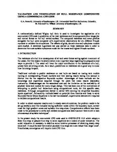
as positive) in predicted values compared to measured values [27]. All statistical and modeling in predictedwere values compared measured values [27]. Allpackage statistical and modeling procedures performed into the R statistical computing (Version 3.2.0). procedures were performed in the R statistical computing package (Version 3.2.0). 3. Results 3. Results 3.1. 3.1. Ground Ground Measurements Measurements and and Parameters Parameters Estimation Estimation All All ground ground measurements measurements data data were were integrated integrated into into 8-day 8-day time time step step for for the the comparability comparability in in temporal resolution with the MODIS data products (Figure 1). Daily Tmin, range from −20.4´20.4 °C to 8.9 ˝C temporal resolution with the MODIS data products (Figure 1). Daily Tmin, range from °C, which was much thethan default upper limit (Tmin_max, 12.02 °C)12.02 in the BPLUT 1 ˝ C, which ˝ C) to 8.9 waslower muchthan lower the default upper limit (Tmin_max, in the(Table BPLUT and Figure In general, VPD fluctuated aroundaround 0.15 ± 0.15 0.10˘(mean ± SD)˘Kpa for a for fewa (Table 1 and1a). Figure 1a). In general, VPD fluctuated 0.10 (mean SD)except Kpa except measurement days accessible to the VPDmin (0.65 Kpa) (Table 1 and Figure 1b). The supreme PAR few measurement days accessible to the VPDmin (0.65 Kpa) (Table 1 and Figure 1b). The supreme PAR appeared on July and August (DOY120-240) that the seasonal average could reach 18.6 ± 4.2 μmol appeared on July and August (DOY120-240) that the seasonal average could reach 18.6 ˘ 4.2 µmol −1 −1 (equal to 4.2 ± 0.9 MJ m−2 day−1) (Figure 1c). photons ´1m−2´day photons m 2 day´1 (equal to 4.2 ˘ 0.9 MJ m´2 day´1 ) (Figure 1c).
Figure variation of of ground ground meteorological meteorologicalmeasurements measurementsdata dataand andthe theFPAR FPAR from 2009 Figure 1. 1. Seasonal Seasonal variation from 2009 to to 2013. All data are integrated into 8-day time step and showed with the first day of each 8-day 2013. All data are integrated into 8-day time step and showed with the first day of each 8-day interval, interval, error bars in (b) (a) and (b) are standard deviation for corresponding mean values. (a), Tmin the errorthe bars in (a) and are standard deviation for corresponding mean values. (a), Tmin is the is theminimum daily minimum temperature; is the pressure daily vapor deficit; (c), PAR is daily temperature; (b), VPD is(b), the VPD daily vapor deficit;pressure (c), PAR is photosynthetically photosynthetically radiation; LAI (d), MG theisconsecutive LAI MG isregression derived from linear regression active radiation; (d),active the consecutive derived from linear between ground LAIG G measurements and MODIS LAI (LAI M ) in LAI G measurement days (n = 23); (e), between ground LAI measurements and MODIS LAI (LAIM ) in LAIG measurement days (n = 23); (e), FPARM is directly M isfrom directly obtained fromwhile MODIS products, while FPARG isGcalculated LAIG in e based FPAR obtained MODIS products, FPARG is calculated from LAI in e basedfrom on Beer-Lambert law. on Beer-Lambert law.
The consecutive LAIMG was stimulated from the linear regression between the consecutive 8-day The consecutive LAIMG was stimulated from the linear regression between the consecutive 8-day time step LAIM and field measurement LAI (LAIG ) in measurement days (LAIMG = 2.33 ˆ LAIM ´ 0.23, time step LAIM and field measurement LAI (LAIG) in measurement days (LAIMG = 2.33 × LAIM − 0.23, R2 = 0.84, p < 0.001, n = 23) (Figure 1d). The LAIM underestimated the vegetation condition in this R2 = 0.84, p < 0.001, n = 23) (Figure 1d). The LAIM underestimated the vegetation condition in this alpine swamp meadow by an average 39.2% except a few days during the non-growing season. The alpine swamp meadow by an average 39.2% except a few days during the non-growing season. The LAIMG reached its maximum on the August with multi-years average 5.99 m2 m´2 (˘0.64 SD) from 2 −2 LAIMG reached its maximum on the August with multi-years average 5.99 m m (±0.64 SD) from 2009 to 2012 (Figure 1d). As Figure 1e illustrated, the FPARM also generally underestimated the 2009 to 2012 (Figure 1d). As Figure 1e illustrated, the FPARM also generally underestimated the
Remote Sens. 2016, 8, 592 Remote Sens. 2016, 8, 592
8 of 19 8 of 18
FPAR G by an average 22.2% during the whole study period. Seasonal FPAR trend was similar to LAI FPARG by an average 22.2% during the whole study period. Seasonal FPAR trend was similar to LAI (Figure 1d,e). (Figure 1d,e). The anan integrated εmaxε estimation of 1.78 g C MJ−1 for ´ this alpine 1 for The MOD17A2 MOD17A2algorithm algorithmcarried carriedout out integrated this max estimation of 1.78 g C MJ 2 wetland from 2009 to 2013 (R = 0.78, p < 0.01, n = 23). Alternatively, the light response curve derived 2 alpine wetland from 2009 to 2013 (R = 0.78, p < 0.01, n = 23). Alternatively, the light response curve from thefrom Michaelis-Menten equation equation providedprovided annual-scale εmax estimation for 1.70, 1.80, 1.33, 1.80, and derived the Michaelis-Menten annual-scale εmax estimation for 1.70, −1 1.59 C MJ 2009 to 2012, (Figure 2a–d and 2a–d Tableand 1). Two max estimate methods ´1 from 1.33,gand 1.59 from g C MJ 2009respectively to 2012, respectively (Figure Tableε1). Two εmax estimate failed to generate significant difference in ε max values (paired t-test, t0.025 = 2.2, df = 4, p = 0.1) during methods failed to generate significant difference in εmax values (paired t-test, t0.025 = 2.2, df = 4, −1 when calculated study we Therefore, assumed the εmax valuethe inε2013value was in 1.78 g C MJ1.78 p = 0.1)period. duringTherefore, study period. we assumed 2013 was g C MJ´1 when max GPP_MODR3 and GPP_MODR4 (Table 1). calculated GPP_MODR3 and GPP_MODR4 (Table 1).
Figure 2. 2. The The maximum thethe light response curve derived from the Figure maximum light lightuse useefficiency efficiencyestimation estimationusing using light response curve derived from Michaelis-Menten equation based on daytime EC measurement data from 2009 to 2012 The Pmax the Michaelis-Menten equation based on daytime EC measurement data from 2009 to (a–d). 2012 (a–d). The ´2 s´1 ) is the maximum ecosystem photosynthesis rate. α (µmol CO µmol photons´1 ) is (µmol CO m −2 −1 2 2 Pmax (μmol CO2 m s ) is the maximum ecosystem photosynthesis rate. α (μmol CO2 μmol photons−1) thethe maximum light use efficiency. is maximum light use efficiency.
Seasonal-Scale Contrast of GPP Estimations 3.2. Seasonal-Scale Seasonal variation variation of of the field GPP measurement (GPP_EC) and five MODIS-based GPP Seasonal estimations (GPP_MOD, (GPP_MOD, GPP_MODR1, GPP_MODR1, GPP_MODR2, GPP_MODR2, GPP_MODR3, GPP_MODR3, and and GPP_MODR4) GPP_MODR4) showed estimations similar tendency but with different quantities in all observational years, especially in growing season GPP_EC was was generally generally greater greater than than any any other other GPP estimation estimation from the MOD17A2 (Figure 3a–e). GPP_EC algorithm, which which indicated indicated that that all MODIS-based MODIS-based GPP GPP estimations estimations in this site were underestimated algorithm, in predicting GPP. GPP_MODR3 got the closest agreement with GPP_EC estimation, GPP_MODR4 took the second place, and the rest MODIS-based GPP estimations (GPP_MOD, GPP_MODR1, and GPP_MODR2) strongly strongly underestimated underestimated GPP GPP in in this this alpine wetland wetland with corresponding values less GPP_MODR2) than half of GPP_EC estimation (Figure 3). In growing season, statistical results showed that the mean GPP estimation from the same method, either the EC-based or the MODIS-based, had no significant differences (p > 0.1) amid different observational years (Table 2). However, diverse estimation methods significantly affected the mean GPP values (p < 0.01) in all observational years (Table 2). In contrast, the GPP_MOD and GPP_MODR1 showed the worst underestimation (less than 35% of GPP_EC), and the GPP_MODR2 came the second
Remote Sens. 2016, 8, 592
9 of 19
(about 40% of GPP_EC). There also existed a significant underestimation (about 64% of GPP_EC) from the GPP_MODR4 despite of significant promotion compared to the former MODIS-based GPP estimation. However, GPP_MODR3 did not show significant difference with GPP_EC (Table 2) thus Remote Sens. 2016, 8, 592 9 of 18 provided an instrumental approach in daily GPP estimation for this alpine wetland.
Figure gross primary production (GPP) estimation fromfrom different methods from Figure 3.3.Seasonal Seasonalvariation variationofof gross primary production (GPP) estimation different methods 2009 2013to(a–e). is from NEE partitioned of EC measurement data, while data, GPP estimations fromto2009 2013GPP_EC (a–e). GPP_EC is from NEE partitioned of EC measurement while GPP based on the based MOD17A2 algorithm are algorithm showed inare Table 1. Datainare 8 days composited GPPcomposited estimation estimations on the MOD17A2 showed Table 1. Data are 8 days showed in the first day. in the first day. GPP estimation showed
In growing season, statistical results showed that the mean GPP estimation from the same Tableeither 2. GPPthe estimation differences diverse estimation and differences inter-annual differences method, EC-based or the among MODIS-based, had nomethods significant (p > 0.1) amid during growing season in different years *. different observational years (Table 2). However, diverse estimation methods significantly affected the mean GPP values (p < 0.01) in all observational years (Table 2). In contrast, the GPP_MOD and 2009 (n = 19) 2010 (n = 18) 2011 (n = 19) 2012 (n = 19) All (n = 75) GPP_MODR1 showed the worst underestimation (less than 35% of GPP_EC), and the GPP_MODR2 GPP_EC 46.91 (˘24.45) Da 45.60 (˘19.41) Ca 37.93 (˘20.52) Ca 40.89 (˘20.50) Ca 40.74 (˘22.39) C came the second13.62 (about 40% There existed a significant underestimation (about 64% GPP_MOD (˘8.91) Aaof GPP_EC). 13.90 (˘9.91) Aa also13.75 (˘8.49) Aa 14.17 (˘9.67) Aa 13.86 (˘9.06) A 10.88 Aa 10.18 (˘4.79)of Aasignificant 11.47 (˘5.09) Aa 11.66 (˘4.65) 10.06 (˘4.78) A ofGPP_MODR1 GPP_EC) from the(˘4.84) GPP_MODR4 despite promotion compared toAa the former MODISGPP_MODR2 15.94 (˘6.55) ABa (˘5.83) ABa 16.18 (˘6.65) Aa 16.49 (˘6.12) ABa 16.01 (˘6.19) A based GPP estimation. However,15.40 GPP_MODR3 did not show significant difference with GPP_EC GPP_MODR3 39.84 (˘16.39) CDa 40.77 (˘15.43) Ca 31.65 (˘13.00) BCa 38.56 (˘14.31) Ca 37.67(˘14.96) C (Table 2) thus provided anBCa instrumental approach in daily GPP for this wetland. GPP_MODR4 27.21 (˘12.11) 26.95 (˘12.69) Ba 22.43 (˘9.96) ABaestimation 27.26 (˘10.86) BCaalpine 25.99 (˘11.46) B * GPP estimation methods are similar to Table 1. Data is the mean (˘1 standard deviation) of 8 days composited GPP estimations. * All raw data of thisamong table passed theestimation normality (Shapiro-Wilk and homogeneity of Table 2. GPP estimation differences diverse methods andtest) inter-annual differences variance test (Bartlett test) (p > 0.05). Statistical analysis is based on the 95% family-wise confidence level during growing season in different years *. (α = 0.05). Rows with the same lowercase indicate no significant difference in different years (p > 0.1), and columns with the different uppercase indicate that a significant difference exist among diverse GPP estimation 2009 (n = 19) 2010 (n = 18) 2011 (n = 19) 2012 (n = 19) All (n = 75) methods (p < 0.01).
GPP_EC 46.91 (±24.45) Da 45.60 (±19.41) Ca 37.93 (±20.52) Ca 40.89 (±20.50) Ca 40.74 (±22.39) C GPP_MOD 13.62 (±8.91) Aa 13.90 (±9.91) Aa 13.75 (±8.49) Aa 14.17 (±9.67) Aa 13.86 (±9.06) A The significant linear regression between EC-based estimation (GPP_EC) MODIS-based GPP_MODR1 10.88 (±4.84) Aa 10.18 (±4.79) Aa 11.47GPP (±5.09) Aa 11.66 (±4.65) Aaand 10.06 (±4.78) A GPP estimation indicated that temporal variation of GPP could be well explained by MODIS-based GPP_MODR2 15.94 (±6.55) ABa 15.40 (±5.83) ABa 16.18 (±6.65) Aa 16.49 (±6.12) ABa 16.01 (±6.19)GPP A GPP_MODR3 CDa n40.77 (±15.43) Ca 4).31.65 (±13.00) BCa 38.56 (±14.31) Ca 37.67(±14.96) C estimation (R2 > 39.84 0.83,(±16.39) p < 0.0001, = 190) (Figure However, the absolute magnitudes of GPP were GPP_MODR4 27.21 (±12.11) BCa 26.95 (±12.69) Ba 22.43 (±9.96) ABa 27.26 (±10.86) BCa 25.99 (±11.46) B undervalued with a attenuation coefficient (slope in the Figure 4) range from 13.0% (GPP_MODR3)
estimation methods are similar to Table 1. Data is the meanwe (±1used standard deviation) of 8 dayswith even *toGPP 75.0% (GPP_MODR1) depending on the methodology (Table 1). In contrast composited GPP estimations. * All raw data of this table passed the normality (Shapiro-Wilk test) and the GPP_MOD estimation, GPP_MODR1 reduced the capacity in the GPP estimation about 10.0% homogeneity of variance test (Bartlett test) (p > 0.05). Statistical analysis is based on the 95% familywise confidence level (α = 0.05). Rows with the same lowercase indicate no significant difference in different years (p > 0.1), and columns with the different uppercase indicate that a significant difference exist among diverse GPP estimation methods (p < 0.01).
The significant linear regression between EC-based GPP estimation (GPP_EC) and MODIS-
Remote Sens. 2016, 8, 592
10 of 18
based GPP estimation (R2 > 0.83, p < 0.0001, n = 190) (Figure 4). However, the absolute magnitudes of GPP were undervalued with a attenuation coefficient (slope in the Figure 4) range from 13.0% Remote Sens. 2016, 8, 592 10 of 19 (GPP_MODR3) even to 75.0% (GPP_MODR1) depending on the methodology we used (Table 1). In contrast with the GPP_MOD estimation, GPP_MODR1 reduced the capacity in the GPP estimation about 10.0%(Figure of GPP_EC (Figure the 4). However, the GPP_MODR2, and GPP_MODR4 of GPP_EC 4). However, GPP_MODR2, GPP_MODR3,GPP_MODR3, and GPP_MODR4 improved the improvedofthe of the GPP 3.0%, 53.0%, and 25.0%,Therefore, respectively. Therefore, accuracy theaccuracy GPP estimations byestimations 3.0%, 53.0%,byand 25.0%, respectively. GPP_MODR3 GPP_MODR3 presented a superiorinperformance in daily GPP estimation compared to other MODISpresented a superior performance daily GPP estimation compared to other MODIS-based models based models (Table Figures 3 and 4). (Table 2, Figures 3 and2,4).
Figure 4. 4. Linear between EC-based EC-based GPP GPP estimation estimation (GPP_EC) (GPP_EC) and and MODIS-based MODIS-based GPP GPP Figure Linear regression regression between estimation. GPP estimations based on the MOD17A2 algorithm are showed in Table 1. (a), GPP_MOD; estimation. GPP estimations based on the MOD17A2 algorithm are showed in Table 1. (a), GPP_MOD; (b), GPP_MODR1; GPP_MODR1; (c), (c), GPP_MODR2; GPP_MODR2; (d), (d), GPP_MODR3; GPP_MODR3; (e), (e), GPP_MODR4. GPP_MODR4. Data days (b), Data are are the the 88 days composited GPP values. The the regression regression curves, curves, the the coverages coverages are are 95% 95% confidence confidence composited GPP values. The solid solid lines lines are are the interval of linear regressions. Dash lines are the 1:1 reference lines. interval of linear regressions. Dash lines are the 1:1 reference lines.
3.3. Annual-Scale of GPP GPP Estimations Estimations 3.3. Annual-Scale Contrast Contrast of −2 Annual GPP_EC 2011 to Annual GPP_EC in in this this alpine alpine wetland wetlandwas wasrange rangefrom fromthe theminimum minimum755.02 755.02ggCCmm´in2 in 2011 −2 in 2010 (Figure 5a). The GPP_MOD had strong underestimation in the maximum 901.37 g C m to the maximum 901.37 g C m´2 in 2010 (Figure 5a). The GPP_MOD had strong underestimation in annual GPP GPP accumulation accumulation that annual that was was only only 27.98% 27.98% in in 2010 2010 to to 34.69% 34.69% in in 2011 2011 of of GPP_EC GPP_EC measurements. measurements. The GPP_MODR1 not only had no improvement in GPP estimation but showed a slight decrease The GPP_MODR1 not only had no improvement in GPP estimation but showed a slight decrease with mean 6.6% of GPP_EC compared with GPP_MOD (Figure 5b). The GPP_MODR1 improved 7.2% with mean 6.6% of GPP_EC compared with GPP_MOD (Figure 5b). The GPP_MODR1 improved 7.2% predictive capacity compared to the GPP_MOD, actually the impact was not significant (Figure 5b). In predictive capacity compared to the GPP_MOD, actually the impact was not significant (Figure 5b). contrast with the GPP_MOD, the GPP_MODR4 had a significant, 31.3% of GPP_EC, promotion in In contrast with the GPP_MOD, the GPP_MODR4 had a significant, 31.3% of GPP_EC, promotion GPP estimation, but there still existed significant difference between GPP_MODR4 and GPP_EC in GPP estimation, but there still existed significant difference between GPP_MODR4 and GPP_EC (Figure 5b). Statistical results showed that there was no significant difference between GPP_MODR3 (Figure 5b). Statistical results showed that there was no significant difference between GPP_MODR3 and GPP_EC, which indicated that the GPP_MODR3 was the most instrumental estimation methods and GPP_EC, which indicated that the GPP_MODR3 was the most instrumental estimation methods in annual GPP accumulation. in annual GPP accumulation.
Remote Sens. 2016, 8, 592 Remote Sens. 2016, 8, 592
11 of 19 11 of 18
Figure 5.5.Inter-annual GPPGPP variations fromfrom the field (GPP_EC) and five and MODISInter-annual variations the GPP fieldmeasurement GPP measurement (GPP_EC) five based GPP estimations (GPP_MOD, GPP_MODR1, GPP_MODR2, GPP_MODR3, and GPP_MODR4) MODIS-based GPP estimations (GPP_MOD, GPP_MODR1, GPP_MODR2, GPP_MODR3, and (a) and the difference different among estimation methods (b). The methods error bars(b). in bThe are error the standard GPP_MODR4) (a) andamong the difference different estimation bars in deviation of the mean annualofGPP estimation to 2012.from The2009 bar with the The same lowercase b are the standard deviation the mean annualfrom GPP2009 estimation to 2012. bar with the indicates no significant difference among diverse GPP estimation methods (p > 0.05). same lowercase indicates no significant difference among diverse GPP estimation methods (p > 0.05).
4. 4. Discussion Discussion This studyutilized utilized MOD17A2 algorithm and tower-based measurements to This study thethe MOD17A2 algorithm and tower-based groundground measurements to reconcile reconcile MODISGPP default GPP estimation (GPP_MOD) in GPP four GPP estimation models, GPP_MODR1 MODIS default estimation (GPP_MOD) in four estimation models, GPP_MODR1 to to GPP_MODR4, depending on the diverse parameterization schemes (Table 1). We assessed the GPP_MODR4, depending on the diverse parameterization schemes (Table 1). We assessed the performance on GPP GPP estimations estimations as as compared compared to to in in situ situ flux flux tower tower GPP GPP (GPP_EC). (GPP_EC). performance of of these these models models on 4.1. Impacts Impacts of of Meteorology Meteorology Data on GPP Estimations In this thisstudy, study,GPP_MOD GPP_MOD strongly underestimated (68.0%) daily GPP meancompared GPP compared to strongly underestimated (68.0%) daily mean to GPP_EC GPP_EC (Table 3 and5). Figure The difference between GPP_MOD andGPP_MODR1 the GPP_MODR1 (Table 3 and Figure The5). difference between GPP_MOD and the was was onlyonly the the meteorology data inputs GPP estimations (Table1).1).Unexpectedly, Unexpectedly, ground ground meteorology meteorology data meteorology data inputs in in GPP estimations (Table (Tmin, VPD, and PAR) used in GPP_MODR1 generated a slightly higher underestimation (RPE of 73.0%) Cm m´−22 than 73.0%) with mean daily RMSE of 2.8 gg C than the the default default DAO DAO data data with with mean mean daily daily RMSE RMSE of ´ 2 −2 that −2.47 g C m caused 6.6% of less integrated estimations in annual mean GPP (Table 2 and Figure 5). ´2.47 g C m that caused 6.6% of less integrated estimations in annual mean GPP (Table 2 and Bulks studies demonstrated that the that DAO data was coarse in theinGPP Figureof 5).previous Bulks of previous studies demonstrated themeteorology DAO meteorology data was coarse the algorithm [25–27,66] that that stems from thethe inaccurate observations ononthree GPP algorithm [25–27,66] stems from inaccurate observations threemeteorological meteorologicalfactors factors of Tmin, VPD, and net surface solar radiation [33,67,68]. [33,67,68]. Turner Turner et al. (2003) (2003) concluded concluded that that the the VPD and minimum performs well when compared to flux flux tower tower measurements measurements minimum temperature temperature data data in in the the DAO performs whereas large positive positive bias, which might might be a reason reason for the the deteriorate deteriorate of GPP_MODR1. GPP_MODR1. whereas PAR has a large However, study also revealed that thethe coarse meteorology datadata in the However, similar similarto toZhang Zhangetetal. al.(2008), (2008),our our study also revealed that coarse meteorology in MOD17 algorithm did not a significant affection in the MODIS GPP products. the MOD17 algorithm didexert not exert a significant affection in the MODIS GPP products. Table 3. Performances of MODIS-based GPP estimations methods on daily GPP estimations as compared to the insitu flux tower GPP (GPP_EC). RMSE (g C m−2) † Methods * GPP_MOD
2009 (n = 46) 2.90
2010 (n = 45) 2.59
2011 (n = 46) 2.14
2012 (n = 45) 2.26
RPE (%) † Mean
2009
2010
2011
2012
Mean
2.47
−70.4
−72.0
−63.7
−65.7
−68.0
Remote Sens. 2016, 8, 592
12 of 19
Table 3. Performances of MODIS-based GPP estimations methods on daily GPP estimations as compared to the insitu flux tower GPP (GPP_EC). RMSE (g C m´2 ) †
RPE (%) †
Methods *
2009 (n = 46)
2010 (n = 45)
2011 (n = 46)
2012 (n = 45)
Mean
2009
2010
2011
2012
Mean
GPP_MOD GPP_MODR1 GPP_MODR2 GPP_MODR3 GPP_MODR4
2.90 3.24 2.84 1.30 2.01
2.59 2.97 2.55 0.95 1.75
2.14 2.41 2.04 0.97 1.55
2.26 2.59 2.21 0.86 1.37
2.47 2.80 2.41 1.02 1.67
´70.4 ´75.1 ´63.8 ´9.4 ´37.9
´72.0 ´77.5 ´66.4 ´11.3 ´40.4
´63.7 ´69.3 ´56.7 ´15.4 ´39.9
´65.7 ´70.0 ´57.8 ´1.4 ´29.9
´68.0 ´73.0 ´61.2 ´9.4 ´37.0
* The MODIS-based GPP estimation methods are similar to Table 1; † The RMSE and RPE are the root mean square error and the relative predictive error between MODIS-based daily GPP estimations and GPP_EC, respectively. The negative RPE represents the underestimation of MODIS-based daily GPP estimations compared to GPP_EC.
4.2. Impacts of εmax on GPP Estimations The default εmax value for grassland in the BPLUT was less than half of the optimized εmax estimations from field observations in this specific biome (Table 1). Validations in parameters of LUE model in most recent studies revealed that the realistic εmax values were undervalued in the MODIS default GPP algorithms [12,25,27,34] with a few exceptions [26], which emphasized the urgent need to reconcile the optimized εmax for more extensive biomes [17,29,35,38,69]. The global look-up table of εmax in the MOD17A2 GPP algorithm is hard to satisfy all vegetation properties due to various biomes with complex climatic, soil types, and associated stand structures and ages [25,28]. Actually, these uncertainties in εmax estimations might also attribute to the practice that LUE is alterable against different cloudiness, generally highest on overcast days and decreases on clear sky days [17], whereas the overcast conditions are not considered in the MOD17 default εmax list and they are assumed to change only with vegetation types [11]. Optimized εmax inputs directly caused that no significant difference was existed between GPP_MODR3 and GPP_EC in daily and annual GPP estimations (Figure 5b and Table 2), which indicated that GPP_MODR3 was an alternative estimation method to evaluate seasonal and annual GPP on this alpine wetland on the Tibetan Plateau. Contrast to GPP_MOD, GPP_MODR3 improved approximately 60% of RPE in the agreements of the model for the insitu flux tower GPP with the lowest RMSE from ´0.86 to ´1.3 g C m´2 (Table 3 and Figure 6). Therefore, refinements of MOD17 εmax may be beneficial to have a more agreeable fit between GPP_EC and MODIS products because optimized εmax inputs directly improve the LUE model for GPP estimation [11,38,39]. 4.3. Impacts of FPAR on GPP Estimations FPAR is an important input variable in light use efficiency model that directly modulates the essential energy source input to photosynthetic systems [9,13,16]. However, FPARM often produce misleading signals in GPP estimations due to the contamination by atmospheric characteristics [28,70]. Thus, compared with FPARM among diverse seasons and different spatial biomes, realistic ground FPARG could be either undervalued [34,71], overvalued [25,29,72], or had a closest agreement [17,34]. In this study, 22.2% (20.4% in 2011 to 23.8% in 2010) of the FPARG derived from ground LAIMG was underestimated by the FPARM (Figure 1d,e). A near study in an alpine meadow, however, demonstrated that the MODIS-based FPAR was about 14.70% higher than the FPARG , which could be attributed that the vegetation canopies in alpine meadow was much less than in this alpine wetland [25,71,73].
evaluate seasonal and annual GPP on this alpine wetland on the Tibetan Plateau. Contrast to GPP_MOD, GPP_MODR3 improved approximately 60% of RPE in the agreements of the model for the insitu flux tower GPP with the lowest RMSE from −0.86 to −1.3 g C m−2 (Table 3 and Figure 6). Therefore, refinements of MOD17 εmax may be beneficial to have a more agreeable fit between GPP_EC products because optimized εmax inputs directly improve the LUE model Remote Sens.and 2016,MODIS 8, 592 13 offor 19 GPP estimation [11,38,39].
Performances of of gross gross primary primary production production (GPP) (GPP) estimation estimation models based on the the MOD17A2 MOD17A2 Figure 6. Performances algorithm compared compared to to in in situ situ flux schemes of of these these algorithm flux tower tower GPP GPP (GPP_EC). (GPP_EC). The The parameterization parameterization schemes models are Table 1. The percentages indicateindicate the improvement of relativeofpredictive models areshowed showedin in Table 1. positive The positive percentages the improvement relative error (RPE) between daily GPP estimations and GPP_EC and vice versa. The solid predictive error (RPE)MODIS-based between MODIS-based daily GPP estimations and GPP_EC and vice versa. The arrows represent algorithm improvements while dashed arrows represent algorithm deterioration. solid arrows represent algorithm improvements while dashed arrows represent algorithm Both the thickness arrow and thearrow intensity the color inofmodel boxes, which boxes, are proportional deterioration. Both of thethe thickness of the andof the intensity the color in model which are to the percentages represent therepresent degree ofthe thedegree modelof performances changes. Thechanges. “Low εmax proportional to the above, percentages above, the model performances The” represents default ε value for grassland in MODIS product, while the “High ε ” represents the max max ” “Low εmax” represents default εmax value for grassland in MODIS product, while the “High εmax natural ε estimations form ground measurements. The “FPAR:ε ” in the central dashed ellipse max max The “FPAR:εmax” in the central represents the natural εmax estimations form ground measurements. shows the interaction of FPAR and εof in GPP models in this alpinein swamp. max dashed ellipse shows the interaction FPAR andestimation εmax in GPP estimation models this alpine swamp.
The improving performance of FPARG inputs, instead of FPARM , into GPP estimation model was different at distinct εmax levels (Figure 6 and Table 3). With the default εmax inputs, although GPP_MODR2 improved the agreement of GPP_MODR1 in daily GPP estimation by 11.8% of RPE with 0.38 g C m´2 decrease in RMSE, the promoting effects was still not significant (Table 3). Nevertheless, when we used the optimized εmax values from our estimation for this specific ecosystem, the effect of the introduction of FPARG (GPP_MODR3) instead of FPARM (GPP_MODR4) would generate an appreciable close to GPP_EC estimation by 27.6% of RPE with 0.58 g C m´2 decrease in RMSE (Table 3). Therefore, the discrepancies of FPAR changes in GPP estimation models among two distinct εmax levels implied that 15.8% of RPE would be related to the interaction of FPAR and εmax (FPAR:εmax ) in GPP estimation models in this alpine swamp [74] (Figure 6). In addition, we also found the same discrepancies (15.8% of RPE) of εmax caused changes in GPP estimation models among two distinct FPAR levels through comparing changes of GPP estimation models from GPP_MODR1 to GPP_MODR4 (36.0% of RPE) and from GPP_MODR2 to GPP_MODR3 (51.8% of RPE) (Figure 6 and Table 3), which confirmed that the FPAR:εmax caused 15.8% of RPE in GPP estimation based on the MOD17A2 algorithm compared to in insitu flux tower GPP (GPP_EC) in this alpine swamp meadow. 4.4. Algorithm Evaluation and Uncertainty In this study, we found the revised MODIS GPP algorithms inordinately improved the GPP estimation quality except for the GPP_MODR1, in which the order of model improvements showed revised εmax (+36.0% of RPE) > FPAR:εmax (+15.8% of RPE) > FPARG (+11.8% of RPE) > meteorology data (´5% of RPE) through the comparisons of model performances (Figures 3–6 and Tables 1–3). Our results coincided with a comparative study in the forest ecosystems of the East Asia that demonstrated the errors of MODIS GPP were mainly caused by uncertainties in εmax and followed by those in FPAR and meteorological data [26]. Meanwhile, many studies pointed out that the improper parameterization of light use efficiency was the most significant limitation of the MOD17 algorithm [14,38,39]. Over an irrigated cropland and an alpine meadow ecosystem, research also confirmed that the underestimation of εmax was the main reason, and the followed was undervalued LAI-caused FPAR, for the considerable underestimation of GPP calculated using the MOD17 algorithm [34]. However, researches in a tropical
Remote Sens. 2016, 8, 592
14 of 19
savanna show that the main reason for the differences between MODIS and tower derived GPP is FPAR, followed by LUE and meteorological inputs [27]. This could be attributed to the different upstream inputs across multiple biomes, artificially high values of MODIS FPAR at low productivity site and relatively low default εmax values at high productivity sites [17], in the LUE estimation procedure [28]. Although GPP_MODR3 predicted the seasonal and annual GPP patterns well and could be treated as an alternative GPP estimation method on this alpine swamp, an approximate 10% of RPE offset in daily GPP estimations still existed (Figures 3–5 and Table 3). Three kinds of reasons could explain this offset and the lager offsets in other MODIS-based GPP estimation models in this study. One is the parameter inputs in MOD17A2 algorithm [34]. First, many relevant researches proposed that the VPD only represents part of the atmospheric evaporative demand but is not entirely representative indicator of water availability condition thus it does not adequately reflect the observational GPP [25,26,35]. Therefore, they advised that soil moisture [17], remote water index [4,15], or precipitation [25] should be added as a stress factor in the MOD17 algorithm to improve GPP simulation [26]. However, in this study, the alpine swamp is waterlogged during the growing season thus the water limitation should not be the main reason for underestimation of MODIS-based GPP. Second, different cloudiness regulated the εmax value changes due to the change of solar radiation intensity, especially the diffuse radiation [75], which have direct or indirect influences on GPP estimation [17]. Moreover, previous studies suggested that light use efficiency should be different between sunlit and shaded leaf due to the distinct acceptance of direct and diffuse radiation [26,35]. Whereas we assumed a constant εmax value for this alpine swamp throughout the year, it also may be a reason for the current offsets in MODIS-based GPP estimation. Another is the uncertainties in temporal-spatial matching between MODIS-based and ground measurements [19]. In the DAO with a spatial resolution of 1˝ ˆ 1.25˝ is hard to perfectly match a 1 km pixel of MODIS products, which may cause large inaccuracies in GPP estimation at spatial scales [19,28]. Besides, the footprint of GPP_EC is not the regular geographical pixel what the MODIS products provide, which implied the inconformity in GPP estimation [29]. In addition, MODIS products outputs an average LAIM with an 8-day time step while LAIG reflects the specific vegetation state in the measurement day, thus the errors of temporal match is also inevitable due to the vegetation activity [11]. The rest is the estimation errors of GPP_EC themselves. The EC measurement exist certain uncertainties caused by instrument malfunction, rainfall, dew formation, and human disturbances [76,77]. Additionally, both the gap filling and NEE partitioning are based on the assumption that the relationship between ecosystem respiration and temperature is similar in all day, daytime and nighttime [57,59,63,78], which may actually produce GPP_EC estimation error [21]. 5. Conclusions In this study, tower-based measurements were used to validate and improve the MODIS-based GPP products in an alpine swamp on the central Tibetan Plateau. Our results indicated that the MOD17 GPP strongly underestimated GPP_EC with a daily mean less than 40% of EC measurements. The large inaccuracies of MODIS GPP were mainly caused by the underestimation of εmax and followed by that of FPAR. The interaction of FPAR:εmax also affected the GPP estimation. We suggested that the suitable εmax for this alpine swamp was about 1.61 g C MJ´1 which was considerably larger than the default 0.68 g C MJ´1 for grassland. The FPARM underestimated 22.2% of the FPARG during the whole study period. However, the DAO meteorology data in the MOD17 algorithm did not exert a significant affection in the MODIS GPP underestimations. Therefore, site-specific optimized parameters inputs, especially εmax and FPARG , are necessary to improve the performance of MOD17 algorithm in GPP estimation, in which the calibrated MOD17A2 algorithm (GPP_MODR3) could explain 91.6% of GPP_EC variance for the alpine swamp meadow. Our results not only improved the accuracy of the site-specific MODIS GPP estimation greatly, but provide a simple approach to quantify GPP more accurately in other similar alpine swamp meadow on the Tibetan Plateau whose
Remote Sens. 2016, 8, 592
15 of 19
field observation was still scanty despite of their extensive lands area and significant position in the winter rangeland for the local livestock. Acknowledgments: We thank the editors and reviewers for their insightful and valuable comments. This work was supported by the National Natural Science Foundation of China (No. 41571042. Name: Quantitative identification on the influence of climate change and human activities in the alpine meadow ecosystem on the Northern Tibet) and the Strategic Priority Research Program of the Chinese Academy of Sciences (No. XDB03030401. Name: Effect of climate warming on alpine shrub and meadow ecosystem on the Tibetan plateau). Author Contributions: Ben Niu, Xianzhou Zhang and Gang Fu conceived and designed the study. Ben Niu, Yongtao He and Gang Fu collected and analyzed the data; Xianzhou Zhang, Yongtao He, Peili Shi and Mingyuan Du contributed observation apparatus; Ben Niu wrote the paper and all other co-authors provided valuable suggestions for the revision. Conflicts of Interest: The authors declare no conflict of interest.
References 1. 2. 3. 4.
5.
6.
7.
8. 9. 10. 11.
12. 13.
14. 15.
Wang, G.X.; Qian, J.; Cheng, G.D.; Lai, Y.M. Soil organic carbon pool of grassland soils on the Qinghai-Tibetan Plateau and its global implication. Sci. Total Environ. 2002, 291, 207–217. Trumbore, S.E.; Bubier, J.L.; Harden, J.W.; Crill, P.M. Carbon cycling in boreal wetlands: A comparison of three approaches. J. Geophys. Res. Atmos. 1999, 104, 27673–27682. [CrossRef] Hirota, M.; Tang, Y.; Hu, Q.; Hirata, S.; Kato, T.; Mo, W.; Cao, G.; Mariko, S. Carbon dioxide dynamics and controls in a deep-water wetland on the Qinghai-Tibetan Plateau. Ecosystems 2006, 9, 673–688. [CrossRef] Gao, Y.; Yu, G.; Yan, H.; Zhu, X.; Li, S.; Wang, Q.; Zhang, J.; Wang, Y.; Li, Y.; Zhao, L.; et al. A MODIS-based photosynthetic capacity model to estimate gross primary production in Northern China and the Tibetan Plateau. Remote Sens. Environ. 2014, 148, 108–118. [CrossRef] MÄKelÄ, A.; Pulkkinen, M.; Kolari, P.; Lagergren, F.; Berbigier, P.; Lindroth, A.; Loustau, D.; Nikinmaa, E.; Vesala, T.; Hari, P. Developing an empirical model of stand GPP with the lue approach: Analysis of eddy covariance data at five contrasting conifer sites in Europe. Glob. Chang. Biol. 2008, 14, 92–108. [CrossRef] Beer, C.; Reichstein, M.; Tomelleri, E.; Ciais, P.; Jung, M.; Carvalhais, N.; Rodenbeck, C.; Arain, M.A.; Baldocchi, D.; Bonan, G.B.; et al. Terrestrial gross carbon dioxide uptake: Global distribution and covariation with climate. Science 2010, 329, 834–838. [CrossRef] [PubMed] Running, S.W.; Thornton, P.E.; Nemani, R.; Glassy, J.M. Global terrestrial gross and net primary productivity from the earth observing system. In Methods in Ecosystem Science; Sala, O.E., Jackson, R.B., Mooney, H.A., Howarth, R.W., Eds.; Springer New York: New York, NY, USA, 2000; pp. 44–57. Zhang, Y.; Wang, C.; Bai, W.; Wang, Z.; Tu, Y.; Yangjaen, D. Alpine wetlands in the Lhasa River Basin, China. J. Geogr. Sci. 2010, 20, 375–388. [CrossRef] Monteith, J.L. Solar radiation and productivity in tropical ecosystems. J. Appl. Ecol. 1972, 9, 747–766. [CrossRef] Olofsson, P.; Eklundh, L.; Lagergren, F.; Jönsson, P.; Lindroth, A. Estimating net primary production for Scandinavian Forests using data from Terra/MODIS. Adv. Space Res. 2007, 39, 125–130. [CrossRef] Heinsch, F.A.; Reeves, M.; Votava, P.; Kang, S.; Milesi, C.; Zhao, M.; Glassy, J.; Jolly, W.M.; Loehman, R.; Bowker, C.F. GPP and NPP (MOD17A2/A3) products NASA MODIS Land Algorithm. Available online: http://giscenter-sl.isu.edu/AOC/AOC_Satellite/MODIS/MOD17UsersGuide.pdf (accessed on 13 July 2016). Sánchez, M.L.; Pardo, N.; Pérez, I.A.; García, M.A. GPP and maximum light use efficiency estimates using different approaches over a rotating biodiesel crop. Agric. For. Meteorol. 2015, 214–215, 444–455. [CrossRef] Potter, C.S.; Randerson, J.T.; Field, C.B.; Matson, P.A.; Vitousek, P.M.; Mooney, H.A.; Klooster, S.A. Terrestrial ecosystem production: A process model based on global satellite and surface data. Glob. Biogeochem. Cycles 1993, 7, 811–841. [CrossRef] Running, S.W.; Nemani, R.R.; Heinsch, F.A.; Zhao, M.; Reeves, M.; Hashimoto, H. A continuous satellite-derived measure of global terrestrial primary production. Bioscience 2004, 54, 547–560. [CrossRef] Xiao, X.; Hollinger, D.; Aber, J.; Goltz, M.; Davidson, E.A.; Zhang, Q.; Moore Iii, B. Satellite-based modeling of gross primary production in an evergreen needleleaf forest. Remote Sens. Environ. 2004, 89, 519–534. [CrossRef]
Remote Sens. 2016, 8, 592
16.
17.
18.
19. 20. 21.
22. 23.
24.
25.
26.
27.
28.
29.
30.
31.
32.
33.
16 of 19
Ruimy, A.; Kergoat, L.; Bondeau, A. Comparing global models of terrestrial net primary productivity (NPP): Analysis of differences in light absorption and light-use efficiency. Glob. Chang. Biol. 1999, 5, 56–64. [CrossRef] Turner, D.P.; Ritts, W.D.; Cohen, W.B.; Gower, S.T.; Running, S.W.; Zhao, M.; Costa, M.H.; Kirschbaum, A.A.; Ham, J.M.; Saleska, S.R.; et al. Evaluation of MODIS NPP and GPP products across multiple biomes. Remote Sens. Environ. 2006, 102, 282–292. [CrossRef] Yuan, W.; Liu, S.; Zhou, G.; Zhou, G.; Tieszen, L.L.; Baldocchi, D.; Bernhofer, C.; Gholz, H.; Goldstein, A.H.; Goulden, M.L.; et al. Deriving a light use efficiency model from eddy covariance flux data for predicting daily gross primary production across biomes. Agric. For. Meteorol. 2007, 143, 189–207. [CrossRef] Zhao, M.; Heinsch, F.A.; Nemani, R.R.; Running, S.W. Improvements of the MODIS terrestrial gross and net primary production global data set. Remote Sens. Environ. 2005, 95, 164–176. [CrossRef] Baldocchi, D. Measuring biosphere-atmosphere exchange of biologically ralated gases with micrometeorological methods. Ecology 1988, 69, 1331–1340. [CrossRef] Reichstein, M.; Falge, E.; Baldocchi, D.; Papale, D.; Aubinet, M.; Berbigier, P.; Bernhofer, C.; Buchmann, N.; Gilmanov, T.; Granier, A.; et al. On the separation of net ecosystem exchange into assimilation and ecosystem respiration: Review and improved algorithm. Glob. Chang. Biol. 2005, 11, 1424–1439. [CrossRef] Hanan, N.P.; Burba, G.; Verma, S.B.; Berry, J.A.; Suyker, A.; Walter-Shea, E.A. Inversion of net ecosystem CO2 flux measurements for estimation of canopy par absorption. Glob. Chang. Biol. 2002, 8, 563–574. [CrossRef] Reichstein, M.; Ciais, P.; Papale, D.; Valentini, R.; Running, S.; Viovy, N.; Cramer, W.; Granier, A.; OgÉE, J.; Allard, V.; et al. Reduction of ecosystem productivity and respiration during the European summer 2003 climate anomaly: A joint flux tower, remote sensing and modelling analysis. Glob. Chang. Biol. 2007, 13, 634–651. [CrossRef] Friend, A.D.; Arneth, A.; Kiang, N.Y.; Lomas, M.; OgÉE, J.; RÖDenbeck, C.; Running, S.W.; Santaren, J.-D.; Sitch, S.; Viovy, N.; et al. Fluxnet and modelling the global carbon cycle. Glob. Chang. Biol. 2007, 13, 610–633. [CrossRef] Fu, G.; Shen, Z.X.; Zhang, X.Z.; Shi, P.L.; He, Y.T.; Zhang, Y.J.; Sun, W.; Wu, J.S.; Zhou, Y.T.; Pan, X. Calibration of MODIS-based gross primary production over an alpine meadow on the Tibetan Plateau. Can. J. Remote Sens. 2012, 38, 157–168. [CrossRef] He, M.; Zhou, Y.; Ju, W.; Chen, J.; Zhang, L.; Wang, S.; Saigusa, N.; Hirata, R.; Murayama, S.; Liu, Y. Evaluation and improvement of MODIS gross primary productivity in typical forest ecosystems of East Asia based on eddy covariance measurements. J. For. Res. 2012, 18, 31–40. [CrossRef] Kanniah, K.D.; Beringer, J.; Hutley, L.B.; Tapper, N.J.; Zhu, X. Evaluation of collections 4 and 5 of the MODIS gross primary productivity product and algorithm improvement at a tropical savanna site in Northern Australia. Remote Sens. Environ. 2009, 113, 1808–1822. [CrossRef] Tang, X.; Li, H.; Huang, N.; Li, X.; Xu, X.; Ding, Z.; Xie, J. A comprehensive assessment of MODIS-derived GPP for forest ecosystems using the site-level fluxnet database. Environ. Earth Sci. 2015, 74, 5907–5918. [CrossRef] Turner, D.P.; Ritts, W.D.; Cohen, W.B.; Maeirsperger, T.K.; Gower, S.T.; Kirschbaum, A.A.; Running, S.W.; Zhao, M.; Wofsy, S.C.; Dunn, A.L.; et al. Site-level evaluation of satellite-based global terrestrial gross primary production and net primary production monitoring. Glob. Chang. Biol. 2005, 11, 666–684. [CrossRef] Verma, M.; Friedl, M.; Richardson, A.; Kiely, G.; Cescatti, A.; Law, B.; Wohlfahrt, G.; Gielen, B.; Roupsard, O.; Moors, E. Remote sensing of annual terrestrial gross primary productivity from MODIS: An assessment using the fluxnet la thuile data set. Biogeosciences 2014, 11, 2185–2200. [CrossRef] Verma, M.; Friedl, M.A.; Law, B.E.; Bonal, D.; Kiely, G.; Black, T.A.; Wohlfahrt, G.; Moors, E.J.; Montagnani, L.; Marcolla, B.; et al. Improving the performance of remote sensing models for capturing intra- and inter-annual variations in daily GPP: An analysis using global fluxnet tower data. Agric. For. Meteorol. 2015, 214–215, 416–429. [CrossRef] Yan, H.; Fu, Y.; Xiao, X.; Huang, H.Q.; He, H.; Ediger, L. Modeling gross primary productivity for winter wheat–maize double cropping system using MODIS time series and CO2 eddy flux tower data. Agric. Ecosyst. Environ. 2009, 129, 391–400. [CrossRef] Yuan, W.; Liu, S.; Yu, G.; Bonnefond, J.-M.; Chen, J.; Davis, K.; Desai, A.R.; Goldstein, A.H.; Gianelle, D.; Rossi, F.; et al. Global estimates of evapotranspiration and gross primary production based on MODIS and global meteorology data. Remote Sens. Environ. 2010, 114, 1416–1431. [CrossRef]
Remote Sens. 2016, 8, 592
34.
35.
36.
37. 38.
39.
40. 41.
42. 43. 44. 45. 46.
47.
48.
49. 50. 51. 52. 53.
17 of 19
Zhang, Y.; Yu, Q.; Jiang, J.I.E.; Tang, Y. Calibration of terra/MODIS gross primary production over an irrigated cropland on the north China plain and an alpine meadow on the Tibetan Plateau. Glob. Chang. Biol. 2008, 14, 757–767. [CrossRef] Zhou, Y.; Wu, X.; Ju, W.; Chen, J.M.; Wang, S.; Wang, H.; Yuan, W.; Andrew Black, T.; Jassal, R.; Ibrom, A.; et al. Global parameterization and validation of a two-leaf light use efficiency model for predicting gross primary production across fluxnet sites. J. Geophys. Res. Biogeosci. 2016, 121, 1045–1072. [CrossRef] Baldocchi, D.; Falge, E.; Gu, L.H.; Olson, R.; Hollinger, D.; Running, S.; Anthoni, P.; Bernhofer, C.; Davis, K.; Evans, R.; et al. Fluxnet: A new tool to study the temporal and spatial variability of ecosystem-scale carbon dioxide, water vapor, and energy flux densities. Bull. Am. Meteorol. Soc. 2001, 82, 2415–2434. [CrossRef] Yu, G.R.; Wen, X.F.; Sun, X.M.; Tanner, B.D.; Lee, X.; Chen, J.Y. Overview of chinaflux and evaluation of its eddy covariance measurement. Agric. For. Meteorol. 2006, 137, 125–137. [CrossRef] Turner, D.P.; Urbanski, S.; Bremer, D.; Wofsy, S.C.; Meyers, T.; Gower, S.T.; Gregory, M. A cross-biome comparison of daily light use efficiency for gross primary production. Glob. Chang. Biol. 2003, 9, 383–395. [CrossRef] Yang, F.; Ichii, K.; White, M.A.; Hashimoto, H.; Michaelis, A.R.; Votava, P.; Zhu, A.X.; Huete, A.; Running, S.W.; Nemani, R.R. Developing a continental-scale measure of gross primary production by combining MODIS and ameriflux data through support vector machine approach. Remote Sens. Environ. 2007, 110, 109–122. [CrossRef] Fensholt, R.; Sandholt, I.; Rasmussen, M.S.; Stisen, S.; Diouf, A. Evaluation of satellite based primary production modelling in the semi-arid sahel. Remote Sens. Environ. 2006, 105, 173–188. [CrossRef] Gitelson, A.A.; Peng, Y.; Masek, J.G.; Rundquist, D.C.; Verma, S.; Suyker, A.; Baker, J.M.; Hatfield, J.L.; Meyers, T. Remote estimation of crop gross primary production with Landsat data. Remote Sens. Environ. 2012, 121, 404–414. [CrossRef] Wang, C.L.; Zhang, Y.L.; Wang, Z.F.; Bai, W.Q. Analysis of landscape characteristics of the wetland systems in the Lhasa River Basin. Resour. Sci. 2010, 32, 1634–1642. He, G.Q.; Yang, G.H.; Feng, Y.Z.; Jiang, Y. Analysis on alpine wetlands eco-system structure and function in Tibet Plateau. Agric. Res. Arid Areas 2007, 25, 185–189. Zhang, Y. Land Use and Land Cover Change and the Climate Change Adaptation in Tibetan Plateau; China Meteorological Press: Beijing, China, 2012. MODIS Collection 5 Global Subsetting and Visualization Tool. Available online: http://daac.ornl.gov/ MODIS (accessed on 12 July 2016). Jenkins, J.P.; Richardson, A.D.; Braswell, B.H.; Ollinger, S.V.; Hollinger, D.Y.; Smith, M.L. Refining light-use efficiency calculations for a deciduous forest canopy using simultaneous tower-based carbon flux and radiometric measurements. Agric. For. Meteorol. 2007, 143, 64–79. [CrossRef] Landsberg, J.J.; Prince, S.D.; Jarvis, P.G.; McMurtrie, R.E.; Luxmoore, R.; Medlyn, B.E. Energy conversion and use in forests: An analysis of forest production in terms of radiation utilisation efficiency (ε). In The Use of Remote Sensing in the Modeling of Forest Productivity; Shimoda, H., Gholz, H.L., Nakane, K., Eds.; Springer Netherlands: Dordrecht, The Netherlands, 1997; pp. 273–298. Fu, G.; Zhang, X.; Zhang, Y.; Shi, P.; Li, Y.; Zhou, Y.; Yang, P.; Shen, Z. Experimental warming does not enhance gross primary production and above-ground biomass in the alpine meadow of Tibet. J. Appl. Remote Sens. 2013, 7, 073505. [CrossRef] Atlas, R.; Lucchesi, R. File Specific for Geos-Das Celled Output; Goddard Space Flight Center: Greenbelt, MD, USA, 2000. Li, C.; He, H.L.; Liu, M.; Su, W.; Fu, Y.L.; Zhang, L.M.; Wen, X.F.; Yu, G.R. The design and application of CO2 flux data processing system at chinaflux. Geo-Inf. Sci. 2008, 10, 557–565. Kaimai, J.C.; Gaynor, J.E. Another look at sonic thermometry. Bound-Lay Meteorol. 1991, 56, 401–410. [CrossRef] Wilczak, J.M.; Oncley, S.P.; Stage, S.A. Sonic anemometer tilt correction algorithms. Bound-Lay Meteorol. 2001, 99, 127–150. [CrossRef] Polsenaere, P.; Lamaud, E.; Lafon, V.; Bonnefond, J.M.; Bretel, P.; Delille, B.; Deborde, J.; Loustau, D.; Abril, G. Spatial and temporal CO2 exchanges measured by eddy covariance over a temperate intertidal flat and their relationships to net ecosystem production. Biogeosciences 2012, 9, 249–268. [CrossRef]
Remote Sens. 2016, 8, 592
54. 55.
56.
57. 58.
59.
60.
61. 62.
63.
64. 65. 66.
67.
68. 69.
70.
71. 72.
73.
18 of 19
Webb, E.K.; Pearman, G.I.; Leuning, R. Correction of flux measurements for density effects due to heat and water-vapor transfer. Q. J. R. Meteorol. Soc. 1980, 106, 85–100. [CrossRef] Leuning, R. The correct form of the webb, pearman and leuning equation for eddy fluxes of trace gases in steady and non-steady state, horizontally homogeneous flows. Bound-Lay Meteorol. 2006, 123, 263–267. [CrossRef] Han, G.; Yang, L.; Yu, J.; Wang, G.; Mao, P.; Gao, Y. Environmental controls on net ecosystem CO2 exchange over a reed (Phragmites australis) wetland in the Yellow River delta, China. Estuar. Coasts 2012, 36, 401–413. [CrossRef] Zhou, L.; Zhou, G.; Jia, Q. Annual cycle of CO2 exchange over a reed (Phragmites australis) wetland in Northeast China. Aquat. Bot. 2009, 91, 91–98. [CrossRef] Reichstein, M.; Tenhunen, J.D.; Roupsard, O.; Ourcival, J.M.; Rambal, S.; Dore, S.; Valentini, R. Ecosystem respiration in two mediterranean evergreen holm oak forests: Drought effects and decomposition dynamics. Funct. Ecol. 2002, 16, 27–39. [CrossRef] Falge, E.; Baldocchi, D.; Olson, R.; Anthoni, P.; Aubinet, M.; Bernhofer, C.; Burba, G.; Ceulemans, G.; Clement, R.; Dolman, H.; et al. Gap filling strategies for long term energy flux data sets. Agric. For. Meteorol. 2001, 107, 71–77. [CrossRef] Ruimy, A.; Jarvis, P.G.; Baldocchi, D.D.; Saugier, B. CO2 fluxes over plant canopies and solar radiation: A review. In Advances in Ecological Research; Begon., I.M., Fitter., A.H., Eds.; Academic Press: Cambridge, MA, USA, 1995; Volume 26, pp. 1–68. Lloyd, J.; Taylor, J.A. On the temperature-dependence of soil respiration. Funct. Ecol. 1994, 8, 315–323. [CrossRef] Van’t Hoff, J.H. Über die zunehmende bedeutung der anorganischen chemie. Vortrag, gehalten auf der 70. Versammlung der gesellschaft deutscher naturforscher und rzte zu düsseldorf. Z. Anorg. Chem. 1898, 18, 1–13. [CrossRef] Lasslop, G.; Reichstein, M.; Papale, D.; Richardson, A.D.; Arneth, A.; Barr, A.; Stoy, P.; Wohlfahrt, G. Separation of net ecosystem exchange into assimilation and respiration using a light response curve approach: Critical issues and global evaluation. Glob. Chang. Biol. 2010, 16, 187–208. [CrossRef] Varlet-Grancher, C.; Bonhomme, R.; Jacob, C.; Artis, P.; Chartier, M. Caracterisation et Evolution de la Structure d'un Couvert Vegetal de Canne a Sucre. Ann. Agron. 1980, 31, 1–26. Zhang, X.Z.; Zhang, Y.G.; Zhoub, Y.H. Measuring and modelling photosynthetically active radiation in Tibet Plateau during April–October. Agric. For. Meteorol. 2000, 102, 207–212. [CrossRef] Zhang, Y.; Song, C.; Sun, G.; Band, L.E.; McNulty, S.; Noormets, A.; Zhang, Q.; Zhang, Z. Development of a coupled carbon and water model for estimating global gross primary productivity and evapotranspiration based on eddy flux and remote sensing data. Agric. For. Meteorol. 2016, 223, 116–131. [CrossRef] Zhao, M.; Running, S.W.; Nemani, R.R. Sensitivity of moderate resolution imaging spectroradiometer (MODIS) terrestrial primary production to the accuracy of meteorological reanalyses. J. Geophys. Res. Biogeosci. 2006, 111. [CrossRef] Olofsson, P.; Van Laake, P.E.; Eklundh, L. Estimation of absorbed par across scandinavia from satellite measurements: Part I: Incident par. Remote Sens. Environ. 2007, 110, 252–261. [CrossRef] Xin, Q.; Broich, M.; Suyker, A.E.; Yu, L.; Gong, P. Multi-scale evaluation of light use efficiency in MODIS gross primary productivity for croplands in the midwestern United States. Agric. For. Meteorol. 2015, 201, 111–119. [CrossRef] Huang, C.; Li, Y.; Yang, H.; Sun, D.; Yu, Z.; Zhang, Z.; Chen, X.; Xu, L. Detection of algal bloom and factors influencing its formation in taihu lake from 2000 to 2011 by MODIS. Environ. Earth Sci. 2013, 71, 3705–3714. [CrossRef] Olofsson, P.; Eklundh, L. Estimation of absorbed par across scandinavia from satellite measurements. Part II: Modeling and evaluating the fractional absorption. Remote Sens. Environ. 2007, 110, 240–251. [CrossRef] Fensholt, R.; Sandholt, I.; Rasmussen, M.S. Evaluation of MODIS lai, fapar and the relation between fapar and NDVI in a semi-arid environment using in situ measurements. Remote Sens. Environ. 2004, 91, 490–507. [CrossRef] Shi, P.L.; Sun, X.M.; Xu, L.L.; Zhang, X.Z.; He, Y.T.; Zhang, D.Q.; Yu, G.R. Net ecosystem CO2 exchange and controlling factors in a steppe—Kobresia meadow on the Tibetan Plateau. Sci. China Ser. D 2006, 49, 207–218. [CrossRef]
Remote Sens. 2016, 8, 592
74. 75.
76. 77.
78.
19 of 19
Kabacoff, R.I. R in Action, Data Analysis and Graphics with r; Manning Publications Co.: Greenwich, CT, USA, 2011. Yuan, W.; Cai, W.; Xia, J.; Chen, J.; Liu, S.; Dong, W.; Merbold, L.; Law, B.; Arain, A.; Beringer, J.; et al. Global comparison of light use efficiency models for simulating terrestrial vegetation gross primary production based on the lathuile database. Agric. For. Meteorol. 2014, 192–193, 108–120. [CrossRef] Saito, M.; Kato, T.; Tang, Y. Temperature controls ecosystem CO2 exchange of an alpine meadow on the northeastern Tibetan Plateau. Glob. Chang. Biol. 2009, 15, 221–228. [CrossRef] Kato, T.; Tang, Y.; Gu, S.; Hirota, M.; Du, M.; Li, Y.; Zhao, X. Temperature and biomass influences on interannual changes in CO2 exchange in an alpine meadow on the Qinghai-Tibetan Plateau. Glob. Chang. Biol. 2006, 12, 1285–1298. [CrossRef] Alberto, M.C.R.; Wassmann, R.; Hirano, T.; Miyata, A.; Kumar, A.; Padre, A.; Amante, M. CO2 /heat fluxes in rice fields: Comparative assessment of flooded and non-flooded fields in the philippines. Agric. For. Meteorol. 2009, 149, 1737–1750. [CrossRef] © 2016 by the authors; licensee MDPI, Basel, Switzerland. This article is an open access article distributed under the terms and conditions of the Creative Commons Attribution (CC-BY) license (http://creativecommons.org/licenses/by/4.0/).