Trace Equivalence Characterization Through Reinforcement Learning

Trace Equivalence Characterization Through Reinforcement Learning Josée Desharnais, Fran¸cois Laviolette, Krishna Priya Darsini Moturu, and Sami Zhioua IFT-GLO, Université Laval, Québec (QC) Canada, G1K-7P4 {first name.last name}@ift.ulaval.ca Abstract. In the context of probabilistic verification, we provide a new notion of trace-equivalence divergence between pairs of Labelled Markov processes. This divergence corresponds to the optimal value of a particular derived Markov Decision Process. It can therefore be estimated by Reinforcement Learning methods. Moreover, we provide some PACguarantees on this estimation.

1

Introduction

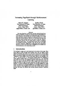
The general field of this research is program verification. Typically, the goal is to check automatically whether a system (program, physical device, protocol, etc.) conforms to its pre-established specification. Both the specification and the implementation are represented using a formal model (generally a transition system) and then a verification algorithm checks for conformance between the two models. This is usually done with the knowledge of the models of the two processes. Our work fits in a more realistic setting where we want to check the conformance between a specification and an implementation (physical device, piece of code, etc.) for which only the model of the specification is available. The model we work with is called a Labelled Markov Process (LMP) [2]; it is a labelled transition systems where transitions are labelled by an action and weighted by a probability (see Figure 1). The action is meant to be synchronized t ttt y tt t • 18 88 b[1] a[1] 88 •3 •4 a[ 12 ]

c[ 12 ]

• 08 88 a[ 12 ] 88 •2 c[1]

•5

•6

a[ 14 ]

•7

•0 a[1]

•1 L L c[ 1 ] x xx b[ 12 ] LLL2L x L& |xx •3 •4 •2 a[ 12 ]

c[ 13 ]

•5

T1

a[ 14 ]

•6 T2

Fig. 1. Labelled Markov Processes

through interaction with the environment. Apart from the modelling of intrinsically probabilistic systems like randomized protocols, probabilities are also used L. Lamontagne and M. Marchand (Eds.): Canadian AI 2006, LNAI 4013, pp. 371–382, 2006. c Springer-Verlag Berlin Heidelberg 2006

372

J. Desharnais et al.

as an abstraction mechanism, for example to hide complex details in suitably chosen probability distributions. The state space of an LMP can be infinite; finite LMPs are also called Probabilistic labelled transition systems or Markov decision processes without rewards. In this paper we will always suppose that it has a tree like representation which, up to bisimulation [2], is always possible. In recent years, a lot of work has been done on pseudo-metrics between probabilistic systems. The reason is that when one wants to compare systems, an equivalence like bisimulation is quite limited: systems are equivalent or they are not. In the presence of probabilities this is even worse because, for one thing, a slight change in the probabilities of equivalent processes will result in non equivalent processes. A pseudometric is an indication of how far systems are. Few pseudometrics have been defined but none of them come with an efficient way to compute it. Moreover, these metrics can only deal with processes whose models are known. This paper is a first step towards the computation of a suitable measure of non equivalence between processes in the presence of unknown models. We have observed that while verification techniques can deal with processes of about 1012 states, Reinforcement Learning (RL) algorithms do a lot better; for example, the TD-Gammon program deals with more than 1040 possible states [13]. Thus we define a divergence notion between LMPs, noted divtrace( . . ), that can be computed with RL algorithms. We call it a divergence rather than a distance because it is not symmetric and does not satisfy the triangle inequality. However, it does have the important property that it is always positive or zero and it is equal to zero if and only if the processes are probabilistic trace-equivalent [9]. Two processes are probabilistic trace-equivalent (we will simply say trace-equivalent) if they accept the same sequences of actions with the same probabilities. For example, T1 and T2 in Figure 1 accept the same traces: ε, a, aa, ab, ac, aac, aca but they are not trace-equivalent since P T1 (aac) = 14 whereas P T2 (aac) = 16 .

2

The Approach

We first informally expose our approach through a one-player stochastic game. Then, we will define a divergence between a specification model (denoted “Spec”) and a real system (denoted “Impl”) for which the model is not available but on which we can interact (exactly as a black-box). This divergence will be the value of the maximal expected reward obtained when playing this game. The formalization and proofs will follow. 2.1

Defining a Game Using Traces

A trace is a sequence of actions (possibly empty) that is meant to be executed on a process. Its execution results in the observation of success or failure of each action1 . For example, if trace aca is executed, then four observations are possible: 1

Note that the execution is sometimes called the trace itself whereas the sequence of actions is called a test.

Trace Equivalence Characterization Through Reinforcement Learning

373

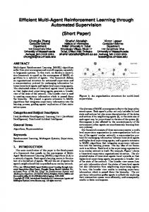
a× , a c× , a c a× and a c a , where a means that a is accepted whereas a× means that it is refused. To each trace is associated a probability distribution on observations. For example, in T2 of Figure 1, the observations related to trace aca have the distribution pa× = 0, pac× = 11 12 = 12 , paca× = 11 12 34 = 38 , paca = 18 . Based on this setting, we have the straightforward result [12]: Proposition 1. Two processes are trace-equivalent iff they yield the same probability distribution on observations for every trace. In the light of this result, a suitable choice to define our divergence could simply be the maximum value, over all traces τ , of the Kullback-Leibler divergence between the probability distributions on observations when running each trace τ on “Spec” and “Impl”. The Kullback-Leibler divergence between two distri1 1 − Eh∼Q ln Q(h) [4]. butions Q and P is defined as KL(QP ) := Eh∼Q ln P (h) Unfortunately, because of the high number of possible traces (on huge systems), the maximum value over all Kullback-Leibler divergences is not tractable. 1 However, Eh∼Q ln Q(h) , the entropy of Q, can be seen as as a quantification over the likeliness to obtain different observations when interacting with “Spec” and a perfect clone of it (which we call “Clone”). “Clone” is simply a copy of the specification but given in the form of a black-box (exactly as “Impl”). In 1 can also be seen as how likely we can obtain different some sense, Eh∼Q ln P (h) observations when interacting (via some τ ) with both “Spec” and “Impl”. Hence, the maximum possible Kullback Leibler divergence should be obtained when executing a suitable trade-off reflecting the fact that the probability of seeing different observations between “Spec” and “Impl” should be as large as possible, and as small as possible between “Spec” and “Clone”. Here is a one-player stochastic game on which a similar tradeoff underlies the optimal solution (see Figure 2). • r 0:::c[1] rr r : y r r •2 • 1 a[ 14 ] :: a[ 24 ] : c[1] : •5 •3 • 4: c[1] :::a[1] •6 •7 Spec a[1]

Impl

Clone

Fig. 2. Implementation, Specification, and Clone

Game0 : The player plays on “Spec”, starting in the initial state; then Step 1 : The player chooses an action a. Step 2 : Action a is run on “Spec”, “Impl” and on a clone of “Spec”. Step 3 : If a succeeds on the three processes, the new player’s state is the reached state in “Spec”; go to Step 1. Else the game ends and the player

374


gets a (+1) reward for different observations between “Spec” and “Impl” added up with a (−1) reward for different observations between “Spec” and “Clone”. That is, writing I for “Impl”, C for “Clone” and Obs for observation, R := (Obs.I = Obs(Spec)) − (Obs(Spec) = Obs.C) where 0 and 1 are used as both truth values and numbers. For example, if action a is executed on the three LMPs and observation F SS is obtained (i.e., Failure in “Impl”, Successes in “Spec” and “Clone”), then an immediate reward of (+1) is given. Notice that once an action fails in one of the three processes the game is stopped. Hence the only scenario allowing to move ahead is: SSS. It is easy to see that if “Spec” and “Impl” are trace-equivalent, the optimal strategy will have expected reward zero, as wanted. Unfortunately the converse is not true: there are trace-inequivalent LMPs for which every strategy has expected reward zero. Here is a counterexample: consider three systems with one a-transition from one state to another one. The probability of this transition is 12 for the “Spec” (and “Clone”) and 1 for the implementation. Thus, the maximal possible expected reward of Game0 will not lead to a notion of trace-equivalence divergence, but we will show that the following slight modification of Game0 does lead to a suitable notion of divergence. Definition 1. Game1 is Game0 with Step 1 replaced by Step 1’ : The player chooses an action and makes a prediction on its success or failure on “Spec” and the reward function is replaced by R := Obs(Spec) = Pred (Obs.I = Obs(Spec)) − (Obs(Spec) = Obs.C) (1) For example, if a is selected and the observation is F SS we obtain a reward of 1((F = S) − (S = S)) = 1 (1 − 0) = 1, but for F F S, we obtain 0 (0 − 1) = 0. Observe that because the player has a full knowledge of what is going on in “Spec”, the prediction in Step 1’ together with this new reward signal gives (implicitly) more control to the player. Indeed, the latter has the possibility to reduce or augment the probability to receive a non zero reward if he expects this reward to be negative or positive. Next section will formalize these ideas in a more Reinforcement Learning setting. 2.2

Constructing the MDP M

In artificial intelligence, Markov Decision Processes (MDPs) offer a popular mathematical tool for planning and learning in the presence of uncertainty [10]. MDPs are a standard formalism for describing multi-stage decision making in probabilistic environments (what we called a one-player stochastic games in the preceding section). The objective of the decision making is to maximize a cumulative measure of long-term performance, called the reward.


375

In an MDP, an agent interacts with an environment at a discrete, low-level time scale. On each time step, the agent observes its current state st ∈ S and chooses an action at from an action set A. One time step later, the agent transits to a new state st+1 , and receives a reward rt+1 . For a given state s and action a, the expected value of the immediate reward is denoted by Rsa S and the transition M to a new state s has probability Prs s (a), regardless of the path taken by the agent before state s (this is the Markov property). The goal in solving MDPs is to find a way of behaving, or policy, which yields a maximal reward. Formally, a policy is defined as a probability distribution for picking actions in each state. For any policy π : S ×A → [0, 1] and any state s ∈ S, the value function of π for state s is defined as the expected infinite-horizon discounted return from s, given that the agent behaves according to π: V π (s) := Eπ {rt+1 +γrt+2 +γ 2 rt+3 +· · · |st = s} where s0 is the initial state and γ is a factor between 0 and 1 used to discount future rewards. The objective is to find an optimal policy, π ∗ which maximizes the value V π (s) of each state s. The optimal value function, V ∗ , is the unique value function corresponding to any optimal policy. If the MDP has finite state and action spaces, and if a model of the environment is known (i.e., immediate rewards Rsa s and transition probabilities PrsMs (a)), then DP algorithms (namely policy evaluation) can compute V π for any policy π. Similar algorithms can be used to compute V ∗ . RL methods, in contrast, compute approximations to V π and V ∗ directly based on the interaction with the environment, without requiring a complete model, which is exactly what we are looking for in our setting. We now define the MDP on which the divergence between two LMPs will be computed. The model of the first LMP, (called “Spec”) is needed and must be in a tree-like representation. It is a tuple (States, s0 , Actions, P rSpec ) where s0 is Spec the initial state and Prs s (a) is the transition probability from state s to state s Spec when action a has been chosen (for example, in Figure 2, Pr1 4 (a) = 24 )). Since it has a tree-like structure, for any state s ∈ States, there is a unique sequence of actions (or trace, denoted tr.s) from s0 to s. For the second LMP (called “Impl”), only the knowledge of all possible conditional probabilities P I(a |τ ) and P I(a× |τ ) of observing the success or failure of an action a given any successfully executed trace τ is required. For example, in Figure 2, P C(c |aa) = 2 2 1 2 C C × 4 ÷ ( 4 + 4 ) = 3 . Finally, we write P (a |τ ) and P (a |τ ) for the conditional probabilities of a copy of the first LMP (called “Clone”): this is for readability and is no additional information since P C(a |τ ) = P S(a |τ )2 . Definition 2. Given “Impl”, “Spec”, and “Clone”, the set of states of the MDP M is S := States ∪ {Dead }, with initial state s0 ; its set of actions is Act := Actions× { , × }. The next-state probability distribution is the same for a and a× (which we represent generically with a- ); it is defined below, followed with the definition of the reward function. 2

Note that the complete knowledge of P I( . | . ) and P C( . | . ) is needed to construct the MDP, but if one only wants to run a Q-learning algorithm on it, only a possibility of interaction with “Clone” and “Impl” is required.

376


Prs s (a) P I(a |tr.s ) P C(a |tr.s ) 1 − P S(a |s) P I(a |tr.s ) P C(a |tr.s ) Spec

M

Prs s (a- ) := Rsa s

0

:=

S

PrsMs (a- )

where • P S(a |s) :=

Δatr.s

P (a |s)

1

-

Spec

s ∈States Prs s × C

if s = Dead if s = Dead

if s = Dead if s = Dead

(a), and P S(a× |s) := 1 − P S(a |s), ×

• Δaτ := P I(a |τ ) P (a |τ ) − P I(a |τ ) P C(a× |τ ) and Δaτ := −Δaτ . The additional Dead state in the MDP indicates the end of an episode and is reached if at least one of the three systems refuses the action. This is witnessed by the next state probability distribution. Let us now see how the reward function Rsa s accords with Game1 presented in the previous section. The simplest case is if the reached state is not Dead : it means that the action succeeded in the three systems (SSS) which indicates a similarity between them. Consequently the reward is zero for both a and a× , as indicated by Step 3 of the game. Let us now consider the case s = Dead. We want the following relation between Rsa s and Rsa S , precisely because the latter represents the average reward of running action a- on a state s: -

-

M

Rsa S = Prs Dead (a- ) RsaDead +

s ∈S\{Dead }

-

M

-

M

Prs s (a- ) Rsa s = Prs Dead (a- ) RsaDead

(2)

0 -

However Game1 and Equation (1) give us another computation for Rsa S . In the case where a- = a is chosen, then the reward is computed only if a succeeds in “Spec”, that is, we get a (+1) reward on observation F SS, a (−1) on SSF , and (+0) on observations SSS or F SF . If a fails, the reward is (+0). Thus,

Rsa S = P I(a× |tr.s) P S(a |s) P C(a |tr.s) − P I(a |tr.s) P S(a |s) P C(a× |tr.s)

F SS → (+1)

= P (a |s) S

SSF → (−1)

Δatr.s .

In the case where a× is chosen, the opposite mechanism is adopted, that is, the reward is computed only if a fails in “Spec” and hence only the situations SF F (+1) and F F S (−1) are relevant. We therefore obtain the following equation: -

-

Rsa S := P S(a- |s) Δatr.s .

(3)

-

The reward RsaDead in Definition 2 is obtained by combining Equations (2) and (3). 2.3

Value of a Policy in M

In order to define a formula for policy evaluations on any state s in our setting, we start from the Bellman Equation [13].


V π (s) =

π(s, a- )

=

Prs s (a- ) (Rsa s + γ V π (s ))

=

-

M

π(s, a- ) (Prs Dead (a- )RsaDead +

a- ∈Act

-

M

s ∈S

a- ∈Act

377

π(s, a- ) (Rsa S +

a- ∈Act

M

s ∈S\{Dead }

-

Prs s (a- )(0 + γ V π (s )))

Prs s (a- ) γ V π (s )) M

(4)

s ∈S\{Dead }

where the second equality follows from Equation (2). Now, let us denote by Si the set of states of S\{Dead} at depth i (i.e., that can be reached from s0 in exactly i steps3 ). We call trace-policy a deterministic (not stochastic) policy for which the same action is selected for states at the same depth. A trace-policy can thus be represented by a trace M+π × × × (s) be the probability to of the MDP (e.g.: π = a 1 a2 a3 a4 a5 ). Let Pj be in s, j steps away from the initial state when following trace-policy π. For example, starting from the LMPs of Figure 2 with traceSpec Spec M+π M+π policy π := a a b , P2 (4) = Pr0 1 (a) Pr1 4 (a) = 24 , but P3 (7) = 0. The - value of the trace-policy π = a1 a2 . . . an on s0 is thus determined as follows from Equation (4): V π (s0 ) =

-

π(s0 , a- ) (Rsa0 S +

a- ∈Act aRs01 S +

= .. . n−1 = = =

i=0 n−1 i=0 n−1

Prs0 s (a- ) γ V π (s )) M

s ∈S\{Dead }

a M Prs0 s (a-1 ) γ Rs2 S + Prs s (a-2 ) γ V π (s )

s ∈S\{Dead }

s ∈S

M

aM+π Pi+1 (s) γ i Rs i+1 S

(5)

s∈Si

γi

a-i+1 M+π Pi+1 (s) P S(a-i+1 |s) Δtr.s

s∈Si

γi

a-

P S(a-i+1 |a1 . . . ai ) Δai+1 1 ...ai

(6)

i=0

Note that there is an abuse of language when we say that a trace-policy is a policy of the MDP, because we assume that after the last action of the sequence, the episode ends even if the Dead state is not reached.

3

Theorems and Definition of divtrace( . . )

We prove in this section that solving the MDP induced by a specification and an implementation yields a trace equivalence divergence between them which is positive and has value 0 if and only if the two processes are trace-equivalent. Let us first state three easy lemmas which will be useful in this section. 3

Since “Spec” is assumed tree-like, the Si ’s are pairwise disjoint.

378


Lemma 1. The following are equivalent. 1. P I(a× |τ ) = P C(a× |τ ). 2. P I(a |τ ) = P C(a |τ ). 3. Δaτ = 0. Lemma 2. Let π = a-1 a-2 . . . a-n be a trace-policy, and τπ = a1 a2 . . . an its corresponding trace. Then for any a- ∈ Act, writing πa- for a-1 a-2 . . . a-n a- , we have πa V (s0 ) = V π (s0 ) iff P I(a- | τπ ) = P C(a- | τπ ) or P S(a- | τπ ) = 0 . -

-

Proof. By Equation (6), we have V πa (s0 ) − V π (s0 ) = γ n Δaτπ P S(a- | τπ ); this implies the result because by Lemma 1, Δaτπ = 0 ⇔ P I(a- | τπ ) = P C(a- | τπ ). Lemma 3. ∀ a- ∈ Act, s ∈ S\{Dead} P S(a- |tr.s) = 0 ⇒ P S(a- | s ) = 0 Proof. Because “Spec” is tree-like, the probability of reaching s by following tr.s is strictly positive. By contraposition, assume that the probability of observing afrom s is strictly positive, then so is the probability of observing a- after tr.s. From now on, we will use the notation a- to mean the opposite of a- , that is, if a- = a then a- = a× and if a- = a× then a- = a . Theorem 1. The following are equivalent: (i) The specification and implementation processes are trace-equivalent. (ii) ∀a- ∈ Act, s ∈ S\{Dead} Rsa S = 0 π (iii) ∀ trace-policy π V (s0 ) = 0 Proof. (i) ⇒ (ii). Since tr.s is a trace ∀ s = Dead, and since P S( . | . ) = P C( . | . ), P S( . | . ) = P I( . | . ) ⇒ ∀a- ∈ Act, s ∈ S\{Dead} P C(a- |tr.s ) = P I(a- |tr.s ) -

⇔ ∀a- ∈ Act, s ∈ S\{Dead} Δatr.s = 0 ⇒ ∀a ∈ Act, s ∈ S\{Dead} -

Rsa S

=0

(by Lemma 1) (by Equation (3))

(ii) ⇒ (i). Let τ be a trace and a- ∈ Act. Case 1: there exists an s ∈ S\{Dead} such that τ = tr.s. Then by (ii) and Equation (3), we have Δatr.s P S(a- |s) = 0. This implies either Δatr.s = 0 or P S(a- |s) = 0. By Lemma 1, we know that the first case implies the result. The second case requires to see the opposite action. Indeed, P S(a- |s) = 0 implies that P S(a- |s) = 1. By (ii), Rsa S = 0. By aS the same argument, we can deduce that either Δtr.s = 0 or P (a |s) = 0, and atherefore that Δtr.s = 0. Since a- = a- , by Lemma 1(replacing a- by a- ), we I C have P (a |tr.s ) = P (a |tr.s ), as wanted. Case 2: if no such s exists, then τ has probability zero in “Spec” and trivially P S(a- |τ ) = 1 = P I(a- |τ ) as wanted. (ii) ⇒ (iii) follows from Equation (5). (iii) ⇒ (ii). Fix a- ∈ Act and s ∈ S\{Dead}, and let n ≥ 0 such that s ∈ Sn , and let a1 . . . an = tr.s. Now, define π = a 1 . . . an . - By (iii) and Equation (6), a-1 ...a-n aπ n we have 0 = 0 − 0 = V (s0 ) − V (s0 ) = γ Δatr.s P S(a- |tr.s ). By Lemma 3, aS Δtr.s P (a |s) = 0, which, by Equation 3, implies the result.


379

Theorem 2. Two LMPs are not trace-equivalent if and only if V π (s0 ) > 0 for some trace-policy π. Proof. (⇒): by Theorem 1, we have that V π (s0 ) = 0 for some trace-policy a-

π = a-1 a-2 . . . a-n . Define J := {j ∈ {1, . . . n} | P C(a-j |a1 . . . aj−1 ) Δaj1 ...aj−1 < 0}, a-

and note that P C(a-j |a1 . . . aj−1 ) > 0 and Δaj1 ...aj−1 < 0 for any j ∈ J. Thus, a-

for any such j, Δaj1 ...aj−1 > 0 (see Definition 2). Let π1 be the policy obtained from π by replacing each action a-j ∈ J by its opposite. Then, by Equation (6), V π1 (s0 ) > 0, as desired. (⇐): follows from Theorem 1. Lemma 4. For every trace-policy π and every a- ∈ Act, -

V π (s0 ) ≤ V πa (s0 ) or V π (s0 ) ≤ V πa (s0 ). -

Proof. As for Theorem 2, the result follows from Equation (6) and the fact that Δτaπ = −Δaτπ where τπ is the trace corresponding to π. Theorem 3. Let M be the MDP induced by “Spec”, “Impl”, and “Clone”. If γ < 1 or |M| < ∞ then V (s0 ) ≥ V π (s0 ) for any trace-policy π. Proof. As explained in the preceding section, a trace policy a-1 . . . a-n is not a policy of M but of the sub-MDP whose state space is S \ ∪∞ i=n+1 Si . If |M| < ∞, the result is a direct consequence of Lemma 4. Otherwise, it is sufficient to show

∀ > 0 ∀ trace-policy π ∃ policy π such that |V π (s0 ) − V π (s0 )| < . of Lemma 4, w.l.o.g., Let > 0 and π = a-1 . . . a-n be a trace-policy. Because ∞ we may suppose n to be large enough to satisfy i=n+1 γ i < . Since on each episode, the reward signal is (−1), (0) or (+1), it is easy to see that any policy π of M that coincides with π on Mπ will have the desired property. We can now give the definition of the central notion of this paper. Definition 3. Let “Spec” and “Impl” be two LMPs and M their induced MDP. We define their trace-equivalence divergence as divtrace(“Spec”“Impl”) := V (s0 ). Clearly, divtrace(“Spec”“Impl”) ≥ 0, and = 0 iff “Spec” and “Impl” are traceequivalent.

4

Implementation and PAC Guarantees

As mentioned in Section 2, the full model of the MDP might not be available. Therefore, it is not appropriate to use a Dynamic Programming [1] algorithm such as value iteration [13] to solve the MDP. Instead, we use a Q-Learning algorithm [15]. Q-Learning is an off-policy Temporal Difference (TD) control algorithm which directly approximates V (s0 ). The algorithm has been proven to converge to the optimal value [8, 14, 16]. Moreover, some results about its

380


convergence rates have been proposed [5]. However, in the field of verification, the main goals are (∗) to find the difference between the implementation of a system and its specification and also (∗∗) to have a guarantee on the fact that this difference is very small in the case where we do not find any such difference during the investigation. Hence, from that perspective, a PAC-guarantee for the Q-Learning algorithm is the most appropriate tool. Definition 4. We say that we have a PAC (Probably Approximately Correct) guarantee for a learning algorithm on an MDP M if, given an a priori precision > 0 and a maximal probability error δ, there exists a function f (M, , δ) such that if the number of episodes is greater than f (M, , δ), then P rob{|V πˆ (s0 ) − V (s0 )| ≤ } ≥ 1 − δ

(7)

where π ˆ is the policy returned by the Q-learning algorithm and V πˆ (s0 ) is the estimation of V (s0 ) given by this algorithm. The Q-learning algorithm does have a PAC guarantee [11], but the function f (M, , δ) is very difficult to compute, which makes this guarantee unusable in practice. The Fiechter RL algorithm [6] comes with a simpler PAC guarantee and hence one can use it in the current setting. The main drawback of the Fiechter algorithm remains its inefficiency compared to Q-Learning. However we can still reach goal (∗) using any RL learning algorithm. Indeed, in the case where the two processes are not trace-equivalent, we can guarantee a bottom bound for the optimal value using Hoeffding inequality [7] based on the following idea. Let π ˆ be the policy returned by the RL algorithm. Let V πˆ (s0 ) be the estimation of V πˆ (s0 ) using a Monte Carlo [13] algorithm with m episodes. Given , δ ∈]0, 1[, according to the Hoeffding inequality, if m ≥ 12 ln( 2δ ), we have Equation (7) with V (s0 ) replaced by V πˆ (s0 ). Since V πˆ (s0 ) never exceeds the optimal value V (s0 ), we have the following PAC guarantee: P rob{V πˆ (s0 ) − V (s0 ) ≤ } ≥ 1 − δ. Note that, in addition, the algorithm returns the policy π ˆ that proves the result. A specific difference between the implementation and its specification is therefore identified, orienting the debugging phase that would follow. This is a major difference with the traditional testing approach consisting of simply running an a priori defined test during the debugging phase. Finally, observe that if V πˆ (s0 ) is too close to zero, or exactly zero, then the Hoeffding inequality gives no guarantee on the trace equivalence or inequivalence. Recall that this difficulty occurs only if we use an algorithm without a tractable PAC guarantee: the problem does not happen with the Fiechter RL algorithm. Nevertheless, even with Q-Learning, we think that our approach is better than traditional testing because, as explained above, it can find new tests by its own. 4.1

Experimental Results

The approach described so far has been implemented using Java. Two action selection algorithms have been experimented: -greedy and SoftMax. For both methods, we tried several functions to decrease the (resp. the τ ) values. The


381

combination that produced the best results is SoftMax such that the temperature k τ is decreasing from 0.8 to 0.01 according to the function : τ = currentEpisod+l (variables k and l are constants). The learning rate α (also called step size) must decrease in order to assure convergence of the Q-Learning algorithm. We tried several decreasing functions and the best convergence results are with x1 where x is the number of times the state-action has been visited. The discount factor γ is fixed to 0.8 in our algorithm. The two following graphics show how the

Q-Learning algorithm converges to the optimal value. This value is, in our setting, the trace-equivalence divergence between the specification and the implementation processes. In the above graphics, we tracked the optimal value in one execution of 10000 episodes. In graphic (a), it is easy to see that the estimated value gets close to the real optimal value (0.132 represented by the line) as the number of episodes increases. Graphic (b), however, is obtained by running the algorithm on trace-equivalent processes. It shows how the estimated value for that case converges to zero.

5

Conclusion

The main contribution of this paper is a completely new approach to estimate how far two LMPs are from being trace-equivalent. Indeed, we introduce a notion of trace-equivalence divergence divtrace( . . ) that can be estimated via some Monte-Carlo estimation using Reinforcement Learning algorithms. Traditional approaches, on the other hand, are based on costly complete calculations on the models. The advantage of using an RL approach therefore opens a way for analyzing very huge systems and even infinite ones. In this paper, we showed that divtrace( . . ) is a real divergence operator and gave some related PAC-guarantees. However, we did not have enough room to show how divtrace( . . ) is increasing as the LMPs are farther from being traceequivalent. This is intuitively clear. The proof, however, is related to the fact

382


that, as for Kullback-Leibler divergence, the divergence Dπ induced by any fixed trace-policy π is of Bregman [3] (here the Bregman function related to Dπ is 1 i∈I xi (1 − 2 xi )). For future work, we want to improve our PAC-guarantees, and even obtain a PAC-guarantee that will not depend on the state space S of the MDP M. We also want to modify the construction of M, in order to speed up the calculation. For example, we could generalize our notion of divergence in a setting where the F F F observation does not stop the episode anymore. Finally, since the LMP formalism is mathematically quite similar to the MDP and HMM (Hidden Markov Model) formalisms, the next step will be to apply our approach on these formalisms.

References 1. R. E. Bellman. Dynamic Programming. Dover Publications, Incorporated, 2003. 2. R. Blute, J. Desharnais, A. Edalat, and P. Panangaden. Bisimulation for labelled Markov processes. In Proc. of the Twelfth IEEE Symposium On Logic In Computer Science, Warsaw, Poland, 1997. 3. Y. Censor. Parallel Optimization: Theory, Algorithms, Applications. Oxford University Press, 1997. 4. T. M. Cover and J. A. Thomas. Elements of Information Theory, chapter 12. Wiley, 1991. 5. E. Even-Dar and Y. Mansour. Learning rates for Q-learning. In COLT ’01/EuroCOLT ’01: Proc. of the 14th Annual Conference on Computational Learning Theory, pages 589–604, London, UK, 2001. Springer-Verlag. 6. C. N. Fiechter. Design and Analysis of Efficient Reinforcement Learning Algorithms. PhD thesis, Univ. of Pittsburgh, 1997. 7. W. Hoeffding. Probability inequalities for sums of bounded random variables. American Statistical Association Journal, 58:13–30, 1963. 8. T. Jaakkola, M. I. Jordan, and S. P. Singh. Convergence of stochastic iterative dynamic programming algorithms. In J. D. Cowan, G. Tesauro, and J. Alspector, editors, Advances in Neural Information Processing Systems, volume 6, pages 703– 710. Morgan Kaufmann Publishers, 1994. 9. C.-C. Jou and S. A. Smolka. Equivalences, congruences, and complete axiomatizations for probabilistic processes. In J.C.M. Baeten and J.W. Klop, editors, CONCUR 90 First International Conference on Concurrency Theory, number 458 in Lecture Notes In Computer Science. Springer-Verlag, 1990. 10. Leslie Pack Kaelbling, Michael L. Littman, and Andrew P. Moore. Reinforcement learning: A survey. Journal of Artificial Intelligence Research, 4:237–285, 1996. 11. M. Kearns and S. Singh. Finite-sample convergence rates for q-learning and indirect algorithms. In Proc. of the 1998 conference on Advances in neural information processing systems II, pages 996–1002, Cambridge, MA, USA, 1999. MIT Press. 12. K. G. Larsen and A. Skou. Bisimulation through probabilistic testing. Inf. Comput., 94(1):1–28, 1991. 13. R. S. Sutton and A. G. Barto. Introduction to Reinforcement Learning. MIT Press, Cambridge, MA, USA, 1998. 14. J. N. Tsitsiklis. Asynchronous stochastic approximation and Q-learning. Machine Learning, 16(3):185–202, 1994. 15. C. Watkins. Learning from Delayed Rewards. PhD thesis, Univ. of Cambridge, 1989. 16. C. Watkins and P. Dayan. Q-learning. Machine Learning, 8:279–292, 1992.