Reinforcement learning through modulation of spike-timing-dependent synaptic plasticity R˘azvan V. Florian Center for Cognitive and Neural Studies (Coneural), Str. Saturn nr. 24, 400504 Cluj-Napoca, Romania Babe¸s-Bolyai University, Institute for Interdisciplinary Experimental Research, Str. T. Laurian nr. 42, 400271 Cluj-Napoca, Romania
[email protected] Abstract The persistent modification of synaptic efficacy as a function of the relative timing of pre- and postsynaptic spikes is a phenomenon known as spiketiming-dependent plasticity (STDP). Here we show that the modulation of STDP by a global reward signal leads to reinforcement learning. We first derive analytically learning rules involving reward-modulated spike-timing-dependent synaptic and intrinsic plasticity, by applying a reinforcement learning algorithm to the stochastic Spike Response Model of spiking neurons. These rules have several features common to plasticity mechanisms experimentally found in the brain. We then demonstrate in simulations of networks of integrateand-fire neurons the efficacy of two simple learning rules involving modulated STDP. One rule is a direct extension of the standard STDP model (modulated STDP), while the other one involves an eligibility trace stored at each synapse that keeps a decaying memory of the relationships between the recent pairs of pre- and postsynaptic spike pairs (modulated STDP with eligibility trace). This latter rule permits learning even if the reward signal is delayed. The proposed rules are able to solve the XOR problem with both rate coded and temporally coded input and to learn a target output firing rate pattern. These learning rules are biologically-plausible, may be used for training generic artificial spiking neural networks, regardless of the neural model used, and suggest the experimental investigation in animals of the existence of reward-modulated STDP. Edited version appeared in Neural Computation 19 (6), pp. 1468-1502, 2007.
1
1 Introduction The dependence of synaptic changes on the relative timing of pre- and postsynaptic action potentials has been experimentally observed in biological neural systems (Markram et al., 1997; Bi and Poo, 1998; Dan and Poo, 2004). A typical example of spike-timing-dependent plasticity (STDP) is given by the potentiation of a synapse when the postsynaptic spike follows the presynaptic spike within a time window of a few tens of milliseconds, and the depression of the synapse when the order of the spikes is reversed. This type of STDP is sometimes called Hebbian, because it is consistent with the original postulate of Hebb that predicted the strengthening of a synapse when the presynaptic neuron causes the postsynaptic neuron to fire. It is also antisymmetric, because the sign of synaptic changes varies with the sign of the relative spike timing. Experiments have also found synapses with anti-Hebbian STDP (where the sign of the changes is reversed, in comparison to Hebbian STDP), as well as synapses with symmetric STDP (Dan and Poo, 1992; Bell et al., 1997; Egger et al., 1999; Roberts and Bell, 2002). Theoretical studies have mostly focused on the computational properties of Hebbian STDP, and have shown its function in neural homeostasis, unsupervised and supervised learning. This mechanism can regulate both the rate and the variability of postsynaptic firing, and may induce competition between afferent synapses (Kempter et al., 1999, 2001; Song et al., 2000). Hebbian STDP can also lead to unsupervised learning and prediction of sequences (Roberts, 1999; Rao and Sejnowski, 2001). Plasticity rules similar to Hebbian STDP were derived theoretically by optimizing the mutual information between the presynaptic input and the activity of the postsynaptic neuron (Toyoizumi et al., 2005; Bell and Parrara, 2005; Chechik, 2003), by minimizing the postsynaptic neuron’s variability to a given input (Bohte and Mozer, 2005), by optimizing the likelihood of postsynaptic firing at one or several desired firing times (Pfister et al., 2006), or by self-repairing a classifier network (Hopfield and Brody, 2004). It was also shown that by clamping the postsynaptic neuron to a target signal, Hebbian STDP can lead, under certain conditions, to learning a particular spike pattern (Legenstein et al., 2005). Anti-Hebbian STDP is, at a first glance, not as interesting as the Hebbian mechanism, as it leads, by itself, to an overall depression of the synapses towards zero efficacy (Abbott and Gerstner, 2005). Hebbian STDP has a particular sensitivity to causality: if a presynaptic neuron contributes to the firing of the postsynaptic neuron, the plasticity mechanism will strengthen the synapse, and thus the presynaptic neuron will become more effective in causing the postsynaptic neuron to fire. This mechanism can determine a network to associate a stable output to a particular input. But let us imagine that the causal relationships are reinforced only when this leads to something good (for example, if the agent controlled by the neural network receives a positive reward), while the causal relationships that lead to failure are weakened, to avoid erroneous behavior. The synapse should feature Hebbian STDP when the reward is positive, and anti-Hebbian STDP when the reward is negative. In this case, the neural network may learn to associate a particular input not to an arbitrary output, determined, e.g., by the initial state of the network, but to a desirable output, 2
as determined by the reward. Alternatively, we may consider the theoretical result that, under certain conditions, Hebbian STDP minimizes the postsynaptic neuron’s variability to a given presynaptic input (Bohte and Mozer, 2005). An analysis analogous to the one performed in that study can show that anti-Hebbian STDP maximizes variability. This kind of influence of Hebbian/anti-Hebbian STDP on variability has also been observed at network level in simulations (Daucé et al., 2005; Soula et al., 2005). By having Hebbian STDP when the network receives positive reward, the variability of the output is reduced and the network could exploit the particular configuration that led to positive reward. By having anti-Hebbian STDP when the network receives negative reward, the variability of the network’s behavior is increased and it could thus explore various strategies until it finds one that leads to positive reward. It is thus tempting to verify whether the modulation of STDP with a reward signal can lead indeed to reinforcement learning, and the exploration of this mechanism is the subject of this paper. This hypothesis is supported by a series of studies on reinforcement learning in non-spiking artificial neural networks, where the learning mechanisms are qualitatively similar to reward-modulated STDP, by strengthening synapses when reward correlates with both presynaptic and postsynaptic activity. The aforementioned studies have focused on networks composed of binary stochastic elements (Barto, 1985; Barto and Anandan, 1985; Barto and Anderson, 1985; Barto and Jordan, 1987; Mazzoni et al., 1991; Pouget et al., 1995; Williams, 1992; Bartlett and Baxter, 1999b, 2000b) or threshold gates (Alstrøm and Stassinopoulos, 1995; Stassinopoulos and Bak, 1995, 1996). These previous results are promising and inspiring, but they do not investigate biologically-plausible reward-modulated STDP, and they use memoryless neurons and work in discrete time. Another study showed that reinforcement learning can be obtained by correlating fluctuations in irregular spiking with a reward signal, in networks composed of neurons firing Poisson spike trains (Xie and Seung, 2004). The resulted learning rule qualitatively resembles reward-modulated STDP as well. However, the results of the study highly depend on the Poisson characteristic of the neurons. Also, this learning model presumes that neurons respond instantaneously, by modulating their firing rate, to their input. This partly ignores the memory of the neural membrane potential, an important characteristic of spiking neural models. Reinforcement learning has also been achieved in spiking neural networks by reinforcement of stochastic synaptic transmission (Seung, 2003). This biologically plausible learning mechanism has several common features with our proposed mechanism, as we will show later, but it is not directly related to STDP. Another existing reinforcement learning algorithm for spiking neural networks requires a particular feed-forward network architecture with a fixed number of layers and is not related to STDP, as well (Takita et al., 2001; Takita and Hagiwara, 2002, 2005). Two other previous studies seem to consider STDP as a reinforcement learning mechanism, but in fact they do not. Strösslin and Gerstner (2003) developed a model for spatial learning and navigation based on reinforcement learning, having as inspiration the hypothesis that eligibility traces are implemented using dopaminemodulated STDP. However, the model does not use spiking neurons, and repre3
sents just the continuous firing rates of the neurons. The learning mechanism resembles just qualitatively to modulated STDP, by strengthening synapses when reward correlates with both presynaptic and postsynaptic activity, as in some other studies already mentioned above. Rao and Sejnowski (2001) have shown that a temporal difference (TD) rule used in conjunction with dendritic backpropagating action potentials reproduces Hebbian STDP. TD learning is often associated with reinforcement learning, where it is used to predict the value function (Sutton and Barto, 1998). But, in general, TD methods are used for prediction problems, and thus implement a form of supervised learning (Sutton, 1998). In the case of the study of Rao and Sejnowski (2001), the neuron learns to predict its own membrane potential, hence it can be interpreted as a form of unsupervised learning since the neuron provides its own teaching signal. In any case, that work does not study STDP as a reinforcement learning mechanism, as there is no external reward signal. In a previous preliminary study, we have derived analytically learning rules involving modulated STDP for networks of probabilistic integrate-and-fire neurons and tested them and some generalizations of them in simulations, in a biologicallyinspired context (Florian, 2005). We have also previously studied the effects of Hebbian and anti-Hebbian STDP in oscillatory neural networks (Florian and Mure¸san, 2006). Here we study in more depth reward-modulated STDP and its efficacy for reinforcement learning. We first derive analytically, in Section 2, learning rules involving reward-modulated spike-timing-dependent synaptic and intrinsic plasticity by applying a reinforcement learning algorithm to the stochastic Spike Response Model of spiking neurons, and discuss the relationship of these rules with other reinforcement learning algorithms for spiking neural networks. We then introduce, in Section 3, two simpler learning rules based on modulated STDP and study them in simulations, in Section 4, to test their efficacy for solving some benchmark problems and to explore their properties. The results are discussed in Section 5. In the course of our study, we found that two other groups have observed independently, through simulations, the reinforcement learning properties of modulated STDP. Soula et al. (2004, 2005) have trained a robot controlled by a spiking neural network to avoid obstacles, by applying STDP when the robot moves forward and anti-Hebbian STDP when the robot hits an obstacle. Farries and Fairhall (2005a,b) have studied a two layer feedforward network where the input units are treated as independent inhomogeneous Poisson processes and output units are single-compartment conductance-based models. The network learned to have a particular pattern of output activity through modulation of STDP by a scalar evaluation of performance. This latter study has been published in abstract form only, and thus the details of the work are not known. In contrast to these studies, in the present paper we also present an analytical justification for introducing rewardmodulated STDP as a reinforcement learning mechanism, and we also study a form of modulated STDP that includes an eligibility trace that permits learning even with delayed reward.
4
2 Analytical derivation of a reinforcement learning algorithm for spiking neural networks In order to motivate the introduction of reward-modulated STDP as a reinforcement learning mechanism, we will derive analytically a reinforcement learning algorithm for spiking neural networks.
2.1 Derivation of the basic learning rule The algorithm is derived as an application of the OLPOMDP reinforcement learning algorithm (Baxter et al., 1999, 2001), an online variant of the GPOMDP algorithm (Bartlett and Baxter, 1999a; Baxter and Bartlett, 2001). GPOMDP assumes that the interaction of an agent with an environment is a partially observable Markov decision process (POMDP), and that the agent chooses actions according to a probabilistic policy µ that depends on a vector w of several real parameters. GPOMDP was derived analytically by considering an approximation to the gradient of the long-term average of the external reward received by the agent with respect to the parameters w. Results related to the convergence of OLPOMDP to local maxima have been obtained (Bartlett and Baxter, 2000a; Marbach and Tsitsiklis, 1999, 2000). It was shown that applying the algorithm to a system of interacting agents that seek to maximize the same reward signal r (t ) is equivalent to applying the algorithm independently to each agent i (Bartlett and Baxter, 1999b, 2000b). OLPOMDP suggests that the parameters w i j (components of the vector wi of agent i ) should evolve according to w i j (t + δt ) = w i j (t ) + γ0 r (t + δt ) z i0j (t + δt ) z i0j (t
+ δt ) = β z i0j (t ) + ζi j (t ) ζi j (t ) =
1
∂µif (t ) i
µif (t ) i
∂w i j
,
(1) (2) (3)
where δt is the duration of a timestep (the system evolves in discrete time), the learning rate γ0 is a small constant parameter, z 0 is an eligibility trace (Sutton and Barto, 1998), ζ is a notation for the change of z 0 resulted from the activity in the last timestep, µif (t ) is the policy-determined probability that agent i chooses action i f i (t ), and f i (t ) is the action actually chosen at time t . The discount factor β is a parameter that can take values between 0 and 1. To accommodate future developments, we made the following changes to standard OLPOMDP notation: β = exp(−δt /τz )
(4)
0
(5)
γ = γ δt /τz z i0j (t ) = z i j (t ) τz ,
5
(6)
with τz being the time constant for the exponential decay of z. We thus have: w i j (t + δt ) = w i j (t ) + γ δt r (t + δt ) z i j (t + δt ) z i j (t + δt ) = β z i j (t ) + ζi j (t ) /τz
(7) (8)
The parameters β and γ0 should be chosen such that δt /(1 − β) and δt /γ0 are large compared to the mixing time τm of the system (Baxter et al., 2001; Baxter and Bartlett, 2001; Bartlett and Baxter, 2000a,c). With our notation and for δt ¿ τz , these conditions are met if τz is large compared to τm and if 0 < γ < 1. The mixing time can be defined rigourously for a Markov process and can be thought of as the time from the occurrence of an action until the effects of that action have died away. We apply this algorithm to the case of a neural network. We consider that at each timestep t , a neuron i either fires ( f i (t ) = 1) with probability p i (t ), or does not fire ( f i (t ) = 0) with probability 1−p i (t ). The neurons are connected through plastic synapses with efficacies w i j (t ), where i is the index of the postsynaptic neuron. The efficacies w i j can be either positive or negative (corresponding to excitatory and inhibitory synapses, respectively). The global reward signal r (t ) is broadcast to all synapses. By considering each neuron i as an independent agent and the firing/nonfiring probabilities of the neuron as determining the policy µi of the corresponding agent (µi1 = p i , µi0 = 1 − p i ), we get the following form of ζi j : 1 ∂p i (t ) , if f i (t ) = 1 p i (t ) ∂w i j ζi j (t ) = 1 ∂p i (t ) , if f i (t ) = 0, − 1 − p i (t ) ∂w i j
(9)
The last equation, together with Eqs. 7 and 8, establishes a plasticity rule that updates the synapses such as to optimize the long term average of the reward received by the network. Up to now, we have followed a derivation also performed by Bartlett and Baxter (1999b, 2000b) for networks of memoryless binary stochastic units, although they called them spiking neurons. Unlike these studies, we consider here spiking neurons where the membrane potential keeps a decaying memory of past inputs, as in real neurons. In particular, we consider the Spike Response Model (SRM) for neurons, that reproduces with high accuracy the dynamics of the complex HodgkinHuxley neural model while being amenable to analytical treatment (Gerstner, 2001; Gerstner and Kistler, 2002). According to the Spike Response Model, each neuron is characterized by its membrane potential u that is defined as X X f u i (t ) = η i (t − tˆi ) + w i j ²i j (t − tˆi , t − t j ), (10) F jt
j
where tˆi is the time of the last spike of neuron i , η i is the refractory response due f to this last spike, t j are the moments of the spikes of presynaptic neuron j emitted 6
f
prior to t , and w i j ²i j (t − tˆi , t − t j ) is the postsynaptic potential induced in neuf
ron i due to an input spike from neuron j at time t j . The first sum runs over all presynaptic neurons, and the last sum runs over all spikes of neuron j prior to t (represented by the set F jt ). We consider that the neuron has a noisy threshold and that it fires stochastically, according to the escape noise model (Gerstner and Kistler, 2002). The neuron fires in the interval δt with probability p i (t ) = ρ i (u i (t ) − θi ) δt , where ρ i is a probability density, also called firing intensity, and θi is the firing threshold of the neuron. We note ∂ρ i = ρ 0i , (11) ∂(u i − θi ) and we have:
∂u i (t ) ∂p i (t ) = ρ 0i (t ) δt . ∂w i j ∂w i j
(12)
From Eq. 10 we get ∂u i (t ) ∂w i j
=
X F jt
f ²i j (t − tˆi , t − t j ),
(13)
hence Eq. 9 can be rewritten as 1 P f if f i (t ) = 1 ρ 0 (t ) F t ²i j (t − tˆi , t − t j ), j ρ i (t ) i ζi j (t ) = δt P f ρ 0i (t ) F t ²i j (t − tˆi , t − t j ), if f i (t ) = 0, − j 1 − ρ i (t ) δt
(14)
Together with Eqs. 7 and 8, this defines the plasticity rule for reinforcement learning. We consider that δt ¿ τz and we rewrite Eq. 8 as τz
z i j (t + δt ) − z i j (t ) δt
= −z i j (t ) + ξi j (t ) + O (
where we noted ξi j (t ) =
ζi j (t ) δt
δt ) z i j (t ), τz
.
(15)
(16)
By taking the limit δt → 0 and using Eqs. 7, 14, 15 and 16, we finally get the reinforcement learning rule for continuous time: dw i j (t ) τz
dt dz i j (t )
= γ r (t ) z i j (t )
(17)
= −z i j (t ) + ξi j (t ) Ã ! X Φi (t ) f ξi j (t ) = − 1 ρ 0i (t ) ²i j (t − tˆi , t − t j ) ρ i (t ) t F dt
j
7
(18) (19)
P f where Φi (t ) = Fi δ(t −t i ) represents the spike train of the postsynaptic neuron as a sum of Dirac functions. f We see that, when a postsynaptic spike emitted at t i follows a presynaptic spike f
f
emitted at t j , z undergoes a sudden growth at t i with f
0 1 ρ i (t i ) f f f ∆z = ²i j (t i − tˆi , t i − t j ) τz ρ i (t f ) i
(20)
that will decay exponentially with a time constant τz . On long term, after the complete decay, this event leads to a total synaptic change ∆w =
Z
∞ f
ti
f
γ r (t ) ∆z exp(−
t − ti τz
) dt
(21)
If r is constant, this is ∆w = γ r ∆z τz . Hence, if r is positive, the algorithm suggests that the synapse should undergo a spike-timing-dependent potentiation, as in experimentally-observed Hebbian STDP. We always have ρ ≥ 0 since it is a probability density and ρ 0 ≥ 0 since the firing probability increases with a higher membrane potential. The spike-timing dependence of the potentiation depends on ² and is approximately exponential, as in experimentally-observed STDP, since ² models the exponential decay of the postsynaptic potential after a presynaptic spike (for more details, see Gerstner and Kistler, 2002). The amplitude of the potentiation is also f f modulated by ρ 0i (t i )/ρ i (t i ), in contrast to standard STDP models, but being consistent with the experimentally observed dependence of synaptic modification not only on relative spike timings, but also on inter-spike intervals (Froemke and Dan, 2002), on which ρ i depends indirectly. Unlike in Hebbian STDP, the depression of z suggested by the algorithm (and the ensuing synaptic depression, if r is positive) is non-associative, as each presynaptic spike decreases z continuously. In general, the algorithm suggests that synaptic changes are modulated by the reinforcement signal r (t ). For example, if the reinforcement is negative, a potentiation of z due to a postsynaptic spike following presynaptic spikes will lead to a depression of the synaptic efficacy w. In the case of constant negative reinforcement, the algorithm implies associative spike-timing-dependent depression and non-associative potentiation of the synaptic efficacy. This type of plasticity has been experimentally discovered in the neural system of the electric fish (Han et al., 2000).
2.2 A neural model for bidirectional associative plasticity for reinforcement learning Since typical experimentally-observed STDP involves only associative plasticity, it is interesting to investigate in which case a reinforcement learning algorithm based
8
on OLPOMDP would lead to associative changes determined by both pre-afterpost and post-after-pre spike pairs. It turns out that this happens when presynaptic neurons homeostatically adapt their firing thresholds to keep the average activity of the postsynaptic neurons constant. To see this, let us consider that not only p i , but also the firing probability p j of presynaptic neuron j depends on the efficacy w i j of the synapse. We apply the OLPOMDP reinforcement learning algorithm to an agent formed by neuron i and all presynaptic neurons j that connect to i . As in the previous case, the policy is parameterized by the synaptic efficacies w i j . However, the policy should now establish the firing probabilities for all presynaptic neurons, as well as for the postsynaptic neuron. Since the firing probabilities depend only on neuronal potentials and thresholds, each neuron decides independently if it fires or not. Hence, the Q j probability of having a given firing pattern f i , { f j } factorizes as µ f i ,{ f j } = µif j µf , i
j
where µkf is the probability of neuron k to choose action f k ∈ {0, 1}. Only µif and i
k
j
µ f depend on w i j and thus j
ζi j (t ) =
1
∂µ f i ,{ f j }
µ f i ,{ f j } ∂w i j
=
µif i
1 Q
³ Q j ´ ∂ µif j µf i
∂w i j
j j µfj
j
=
1 µif i
j µf j
´ ³ j ∂ µif µ f i
∂w i j
j
(22)
The particular form of ζi j depends on the various possibilities for the actions taken by neurons i and j : (1 − p i )(1 − p j ), if f i = f j = 0 j (23) µif i µ f = p i (1 − p j ), if f i = 1 and f j = 0 j (1 − p i ) p j , if f i = 0 and f j = 1 We do not consider the case f i = f j = 1 since there is a negligibly small probability to have simultaneous spiking in a very small interval δt . After performing the calculation of ζi j for the various cases and considering that δt → 0, by analogy with Eq. 9 and the calculation from the previous section, we get: µ ¶ µ ¶ Φ j (t ) ∂ρ j (t ) Φi (t ) ∂ρ i (t ) ξi j (t ) = −1 + −1 (24) ρ i (t ) ∂w i j ρ j (t ) ∂w i j Let us consider that the firing threshold of neuron j has the following dependence: X X f θ j (t ) = θ j w k j χ j (t − t k ) , (25) Fkt
k
where θ j is an arbitrary continuous increasing function, the first sum runs over all postsynaptic neurons to which neuron j projects and the second sum runs over all spikes prior to t of postsynaptic neuron k. χ j is a decaying kernel; for example, ³ ´ f f χ j (t − t k ) = exp −(t − t k )/τθ j , which means that θ j depends on a weighed estimate of the firing rate of postsynaptic neurons, computed using an exponential kernel with time constant τθ j . 9
The proposed dependence of presynaptic firing thresholds means that when the activity of postsynaptic neurons is high, the neuron j increases its firing threshold in order to contribute less to their firing and decrease their activity. The activity of each neuron k is weighed with the synaptic efficacy w k j , since an increase in the firing threshold and a subsequent decrease of the activity of neuron j will have a bigger effect on postsynaptic neurons to which synaptic connections are strong. This is biologically-plausible, since there are many neural mechanisms that ensure homeostasis (Turrigiano and Nelson, 2004) and plasticity of intrinsic excitability (Daoudal and Debanne, 2003; Zhang and Linden, 2003), including mechanisms that regulate the excitability of presynaptic neurons as a function of postsynaptic activity (Nick and Ribera, 2000; Ganguly et al., 2000; Li et al., 2004). The firing intensity of neuron j is ρ j (t ) = ρ j (u j (t ) − θ j (t )). We have ∂ρ j (t ) ∂w i j
= −ρ 0j (t )
∂θ j (t ) ∂w i j
= −ρ 0j (t )θ 0j (t )
X Fit
f
χ j (t − t i ).
(26)
We finally have à ξi j (t ) =
Φi (t ) ρ i (t )
à −
! − 1 ρ 0i (t )
Φ j (t ) ρ j (t )
X F jt
f ²i j (t − tˆi , t − t j )+
! + 1 ρ 0j (t ) θ 0j (t )
X Fit
f
χ j (t − t i ),
(27)
which together with Eqs. 17 and 18 define the plasticity rule in this case. We have the same associative spike-timing-dependent potentiation of z as in the previous case, but now we also have an associative spike-timing-dependent f depression of z. The depression corresponding to a presynaptic spike at t j followf
ing a postsynaptic spike at t i is f
0 1 ρ j (t j ) 0 f f f ∆z = − θ (t ) χ j (t j − t i ), τz ρ j (t f ) j j j
(28)
and the dependence on the relative spike timing is given by χ j . The variation of z is negative because ρ 0j and θ 0j are positive since they are derivatives of increasing functions, ρ j is positive since it is a probability density, and χ j is positive by definition. We have thus shown that a bidirectional associative spike-timing-dependent plasticity mechanism can result from a reinforcement learning algorithm applied to a spiking neural model with homeostatic control of the average postsynaptic activity. As previously, the synaptic changes are modulated by the global reinforcement signal r (t ). As in the previous case, we also have non-associative changes of z: each presynaptic spike depresses z continuously, while each postsynaptic spike potentiates z continuously. However, depending on the parameters, the non-associative changes 10
may be much smaller than the spike-timing-dependent ones. For example, the magnitude of non-associative depression induced by presynaptic spikes is modulated with the derivative (with respect to the difference between the membrane potential and the firing threshold) of the postsynaptic firing intensity, ρ 0i . This usually has a non-negligible value when the membrane potential is high (see the forms of the ρ function from (Gerstner and Kistler, 2002; Bohte, 2004)) and thus a postsynaptic spike is probable to follow. When this happens, z is potentiated and the effect of the depression may be overcome.
2.3 Reinforcement learning and spike-timing-dependent intrinsic plasticity In this section, we consider that the firing threshold θi of the postsynaptic neuron is also an adaptable parameter that contributes to learning, like the w i j parameters. There is ample evidence that this is the case in the brain (Daoudal and Debanne, 2003; Zhang and Linden, 2003). The firing threshold will change according to dθi (t ) = γθ r (t ) z i θ (t ) (29) dt dz i θ (t ) τzθ = −z i θ (t ) + ξi θ (t ) (30) dt 1 1 ∂p i (t ) , if f i (t ) = 1 δt p i (t ) ∂θi ξi θ (t ) = limδt →0 (31) 1 1 ∂p i (t ) − , if f i (t ) = 0, δt 1 − p i (t ) ∂θi by analogy with Eqs. 17, 18, 9 and 19. Since ∂p i (t )/∂θi = −ρ 0i (t ) δt , we have ¶ µ Φi (t ) ξi θ (t ) = − + 1 ρ 0i (t ) ρ i (t )
(32)
Hence, for positive reward, postsynaptic spikes lead to a decrease of the postsynaptic firing threshold (an increase of excitability). This is consistent with experimental results that showed that neural excitability increases after bursts (Aizenman and Linden, 2000; Cudmore and Turrigiano, 2004; Daoudal and Debanne, 2003). Between spikes, the firing threshold increases continuously (but very slowly when the firing intensity, and thus also its derivative with respect to the difference between the membrane potential and the firing threshold, is low). This reinforcement learning algorithm using spike-timing-dependent intrinsic plasticity is complementary with the two other algorithms previously described, and can work simultaneously with any of them.
2.4 Relationship to other reinforcement learning algorithms for spiking neural networks It can be shown that the algorithms proposed here share a common analytical background with the other two existing reinforcement learning algorithms for generic 11
spiking neural networks (Seung, 2003; Xie and Seung, 2004). Seung (2003) applies OLPOMDP by considering that the agent is a synapse, instead of a neuron, as we did. The action of the agent is the release of a neurotransmitter vesicle, instead of the spiking of the neuron, and the parameter that is optimized is a parameter that controls the release of the vesicle, instead of the synaptic connections to the neuron. The result is a learning algorithm that is biologically plausible, but for which there exists no experimental evidence yet. Xie and Seung (2004) do not model in detail the integrative characteristics of the neural membrane potential, and consider that neurons respond instantaneously to inputs by changing the firing rate of their Poisson spike train. Their study derives an episodic algorithm that is similar to GPOMDP, and extends it to an online algorithm similar to OLPOMDP without any justification. The equations determining online learning, Eqs. 16 and 17 in (Xie and Seung, 2004), are identical, after adapting notation, to the ones in our paper, Eqs. 17, 18 and 19. By reinterpreting the current-discharge function f in (Xie and Seung, 2004) as the firing intensity ρ, and the synaptic current h i j as the postsynaptic kernel ²i j , we can see that the algorithm of Xie and Seung is mathematically equivalent to the algorithm derived, more accurately, here. However, our different interpretation and implementation of the mathematical framework permits making better connections to experimentally observed STDP and also a straightforward generalization and application to neural models commonly used in simulations, which the Xie and Seung algorithm does not permit because of the dependence on the memoryless Poisson neural model. The common analytical background of all these algorithms suggests that their learning performance should be similar. Pfister et al. (2006) developed a theory of supervised learning for spiking neurons that leads to STDP and that can be reinterpreted in the context of reinforcement learning. They studied in detail only particular, episodic learning scenarios, not the general, online case approached in our paper. However, the analytical background is again the same one, since in their work synaptic changes depend on a quantity (Eq. 7 in their paper) that is the integral over the learning episode of our ξi j (t ), Eq. 19. It is thus not surprising that some of their results are similar to ours: they find a negative offset of the STDP function that corresponds to the non-associative depression suggested by our algorithm for positive reward, and they derive associative spike-timing dependent depression as the consequence of a homeostatic mechanism, as we did in a different framework.
3 Modulation of STDP by reward The derivations in the previous sections show that reinforcement learning algorithms that involve reward-modulated STDP can be justified analytically. We have also previously tested in simulation, in a biologically-inspired experiment, one of the derived algorithms, to demonstrate practically its efficacy (Florian, 2005). However, these algorithms involve both associative spike-timing-dependent synaptic changes and non-associative ones, unlike standard STDP (Bi and Poo, 1998; Song
12
et al., 2000), but in agreement with certain forms of STDP observed experimentally (Han et al., 2000). Moreover, the particular dynamics of the synapses depends on the form of the firing intensity ρ, which is a function for which there exists no experimentally justified model. For these reasons, we chose in the following to study in simulations some simplified forms of the algorithms derived analytically, that extend in a straightforward way the standard STDP model. The learning rules that we propose below can be applied to any type of spiking neural model; their applicability is not restricted to probabilistic models nor to the SRM model that we previously used in the analytical derivation. The proposed rules are just inspired by the analytically derived and experimentally observed ones, and do not follow directly from them. In what follows, we drop the dependence of plasticity on the firing intensity (which means that the learning mechanism can also be applied to deterministic neural models commonly used in simulations), we consider that both potentiation and depression of z are associative and spike-timing-dependent (without considering the homeostatic mechanism introduced in Section 2.2), we use an exponential dependence of plasticity on the relative spike timings, and we consider that the effect of different spike pairs is additive, as in previous studies (Song et al., 2000; Abbott and Nelson, 2000). The resulting learning rule is determined by Eqs. 17 and 18, which we repeat below for convenience, and an equation for the dynamics of ξ that takes into account these simplifications: dw i j (t ) τz
dt dz i j (t ) dt
= γ r (t ) z i j (t )
(33)
= −z i j (t ) + ξi j (t )
(34)
ξi j (t ) = Φi (t ) A +
X
exp −
f
t − tj
F jt
τ+
+ Φ j (t ) A −
à X Fit
exp −
f
t − ti τ−
! ,
(35)
where τ± and A ± are constant parameters. The time constants τ± determine the ranges of interspike intervals over which synaptic changes occur. According to the standard antisymmetric STDP model, A + is positive and A − is negative. We call the learning rule determined by the above equations modulated STDP with eligibility trace (MSTDPET). The learning rule can be simplified further by dropping the eligibility trace. In this case, we have a simple modulation by the reward r (t ) of standard STDP: dw i j (t ) dt
= γ r (t ) ξi j (t ),
(36)
where ξi j (t ) is given by Eq. 35. We call this learning rule modulated STDP (MSTDP). We remind that, with our notation, the standard STDP model is given by dw i j (t ) dt
= γ ξi j (t ).
(37)
For all these learning rules, it is useful to introduce a variable P i+j that tracks the influence of presynaptic spikes and a variable P i−j that tracks the influence of 13
postsynaptic spikes, instead of keeping in memory, in computer simulations, all past spikes and summing repeatedly their effects (Song et al., 2000). These variables may have biochemical counterparts in biological neurons. The dynamics of ξ and P ± is then given by: ξi j (t ) = P i+j Φi (t ) + P i−j Φ j (t ) dP i+j /dt dP i−j /dt
= −P i+j /τ+ = −P i−j /τ−
(38)
+ A + Φ j (t )
(39)
+ A − Φi (t )
(40)
If τ± and A ± are identical for all synapses, as it is the case in our simulations, then P i+j does not depend on i and P i−j does not depend on j , but we will keep the two indices for clarity. If we simulate the network in discrete time with a timestep δt , the dynamics of the synapses is defined, for MSTDPET, by Eqs. 7 and 8, or, for MSTDP, by w i j (t + δt ) = w i j (t ) + γ r (t + δt ) ζi j (t ),
(41)
and by ζi j (t ) P i+j (t ) P i−j (t )
=
P i+j (t ) f i (t ) + P i−j (t ) f j (t )
(42)
=
P i+j (t P i−j (t
− δt ) exp(−δt /τ+ ) + A + f j (t )
(43)
− δt ) exp(−δt /τ− ) + A − f i (t ),
(44)
=
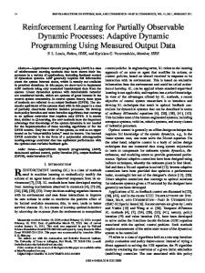
where f i (t ) is 1 if neuron i has fired at timestep t or 0 otherwise. The dynamics of the various variables is illustrated in Fig. 1. As for the standard STDP model, we also apply bounds to the synapses, additionally to the dynamics specified by the learning rules.
4 Simulations 4.1 Methods In the following simulations we used networks composed of integrate-and-fire neurons with resting potential u r = −70 mV, firing threshold θ = −54 mV, reset potential equal to the resting potential, and decay time constant τ = 20 ms (parameters from (Gütig et al., 2003) and similar to those in (Song et al., 2000)). The network’s dynamics was simulated in discrete time with a timestep δt = 1 ms. The synaptic weights w i j represented the total increase of the postsynaptic membrane potential caused by a single presynaptic spike; this increase was considered to take place during the timestep following the spike. Thus, the dynamics of the neurons’ membrane potential was given by X u i (t ) = u r + [u i (t − δt ) − u r ] exp(−δt /τ) + w i j f j (t − δt ) (45) j
If the membrane potential surpassed the firing threshold θ, it was reset to u r . Axons propagated spikes with no delays. More biologically-plausible simulations of 14
1 0 1 fi 0 1.5 + Pij , Pij -1.5 1.5 ζ ij -1.5 1.5 zij -1.5 1.5 r -1.5 w ij 0.5 (MSTDPET) 0.1 0.5 w ij (MSTDP) 0.1 0.5 w ij (STDP) 0.1 0 fj
50
100 Time (ms)
150
200
Figure 1: An illustration of the dynamics of the variables used by MSTDP and MSTDPET, and the effects of these rules and of STDP on the synaptic strength, for sample spike trains and reward (see Eqs. 7, 8, 41, 42, 43, 44). We used γ = 0.2; the values of the other parameters are listed in Section 4.1.
15
reward-modulated STDP were presented elsewhere (Florian, 2005); here, we aim to present the effects of the proposed learning rules using minimalist setups. We used τ+ = τ− = 20 ms; the value of γ varied from experiment to experiment. Except where specified, we used τz = 25 ms, A + = 1 and A − = −1.
4.2 Solving the XOR problem: Rate coded input We first show the efficacy of the proposed rules for learning XOR computation. Although this is not a biologically-relevant task, it is a classic benchmark problem for artificial neural network training. This problem was also approached using other reinforcement learning methods for generic spiking neural networks (Seung, 2003; Xie and Seung, 2004). XOR computation consists in performing the following mapping between two binary inputs and one binary output: {0, 0} → 0 ; {0, 1} → 1 ; {1, 0} → 1 ; {1, 1} → 0 . We considered a setup similar to the one in (Seung, 2003). We simulated a feedforward neural network with 60 input neurons, 60 hidden neurons and one output neuron. Each layer was fully connected to the next layer. Binary inputs and outputs were coded by the firing rates of the corresponding neurons. The first half of the input neurons represented the first input, and the rest the second input. The input 1 was represented by a Poisson spike train at 40 Hz, while the input 0 was represented by no spiking. The training was accomplished by presenting the inputs and then delivering the appropriate reward or punishment to the synapses, according to the activity of the output neuron. In each learning epoch, the four input patterns were presented for 500 ms each, in random order. During the presentation of each input pattern, if the correct output was 1, the network received a reward r = 1 for each output spike emitted and 0 otherwise. This rewarded the network for having a high output firing rate. If the correct output was 0, the network received a negative reward (punishment) r = −1 for each output spike and 0 otherwise. The corresponding reward was delivered during the timestep following the output spike. 50% of the input neurons coding for either inputs were inhibitory, the rest were excitatory. The synaptic weights w i j were hard bounded between 0 and 5 mV (for excitatory synapses) or between -5 mV and 0 (for inhibitory synapses). Initial synaptic weights were generated randomly within the specified bounds. We considered that the network learned the XOR function if, at the end of an experiment, the output firing rate for the input pattern {1, 1} was lower than the output rates for the patterns {0, 1} or {1, 0} (the output firing rate for the input {0, 0} was obviously always 0). Each experiment included 200 learning epochs (presentations of the four input patterns), corresponding to 400 s of simulated time. We investigated learning with both MSTDP (using γ = 0.1 mV) and MSTDPET (using γ = 0.625 mV). We found that both rules were efficient for learning the XOR function (Fig. 2). The synapses changed such as to increase the reward received by the network, by minimizing the firing rate of the output neuron for the input pattern {1, 1} and maximizing the same rate for {0, 1} and {1, 0}. With MSTDP, the network learned the task in 99.1% of 1000 experiments, while with MSTDPET learning was achieved in 98.2% of the experiments. 16
MSTDP
MSTDPET
250
a)
Reward
200 150 100 50
Average Sample
0 -50
0
50
100
150
b)
Average firing rate (Hz)
Learning epoch
200 0
50
100
150
200
Learning epoch
300 250 200 150 100 50 0
{0,0}
{0,1}
{1,0}
{1,1}
Input pattern
{0,0}
{0,1}
{1,0}
{1,1}
Input pattern
Figure 2: Learning XOR computation with rate coded input with MSTDP and MSTDPET. a) Evolution during learning of the total reward received in a learning epoch: average over experiments and a random sample experiment. b) Average firing rate of the output neuron after learning (total number of spikes emitted during the presentation of each pattern in the last learning epoch divided by the duration of the pattern): average over experiments and standard deviation.
17
a)
Reward
MSTDP 35 30 25 20 15 10 5 0 -5
MSTDPET
Average Sample 0
50
100
150
200 0
50
Learning epoch
100
150
200
Learning epoch
b)
Average firing rate (Hz)
100 80 60 40 20 0
{0,0}
{0,1}
{1,0}
{1,1}
Input pattern
{0,0}
{0,1}
{1,0}
{1,1}
Input pattern
Figure 3: Learning XOR computation with temporally coded input with MSTDP and MSTDPET. a) Evolution during learning of the total reward received in a learning epoch: average over experiments and a random sample experiment. b) Average firing rate of the output neuron after learning (total number of spikes emitted during the presentation of each pattern in the last learning epoch divided by the duration of the pattern): average over experiments and standard deviation.
The performance in XOR computation remained constant, after learning, if the reward signal was removed and the synapses were fixed.
4.3 Solving the XOR problem: Temporally coded input Since in the proposed learning rules synaptic changes depend on the precise timing of spikes, we investigated whether the XOR problem can also be learned if the input is coded temporally. We used a fully connected feed-forward network with 2 input neurons, 20 hidden neurons and one output neuron, a setup similar to the one in (Xie and Seung, 2004). The input signals 0 and 1 were coded by two distinct spike trains of 500 ms in length, randomly generated at the beginning of each experiment by distributing uniformly 50 spikes within this interval. Thus, to underline the distinction with rate coding, all inputs had the same average firing rate 18
of 100 Hz. Since the number of neurons was low, we did not divide them into excitatory and inhibitory ones, and allowed the weights of the synapses between input and the hidden layer to take both signs. These weights were bounded between -10 mV and 10 mV. The weights of the synapses between the hidden layer and the output neuron were bounded between 0 and 10 mV. As before, each experiment consisted in 200 learning epochs, corresponding to 400 s of simulated time. We used γ = 0.01 mV for experiments with MSTDP, and γ = 0.25 mV for MSTDPET. With MSTDP, the network learned the XOR function in 89.7% of 1000 experiments, while with MSTDPET learning was achieved in 99.5% of the experiments (Fig. 3). The network learned to solve the task by responding to the synchrony of the two input neurons. We verified that, after learning, the network solves the task not only for the input patterns used during learning, but for any pair of random input signals similarly generated.
4.4 Learning a target firing rate pattern We have also verified the capacity of the proposed learning rules to allow a network to learn a given output pattern, coded by the individual firing rates of the output neurons. During learning, the network received a reward r = 1 when the distance d between the target pattern and the actual one decreased, and a punishment r = −1 when the distance increased, r (t + δt ) = sign(d (t ) − d (t − δt )). We used a feedforward network with 100 input neurons directly connected to 100 output neurons. Each output neuron received axons from all input neurons. Synaptic weights were bounded between 0 and w max = 1.25 mV. The input neurons fired Poisson spike trains with constant, random firing rates, generated uniformly, for each neuron, between 0 and 50 Hz. The target firing rates ν0i of individual output neurons were also generated randomly at the beginning of each experiment, uniformly between 20 and 100 Hz. The actual firing rates νi of the output neurons were measured using a leaky integrator with time constant τν = 2 s: νi (t ) = νi (t − δt ) exp(−
δt 1 )+ f i (t ). τν τν
(46)
This is equivalent to performing a weighed estimate of the firing rate with an exponential kernel. We measured the totalq distance between the current output firing P 0 2 pattern and the target one as d (t ) = i [νi (t ) − νi ] . Learning began after the output rates stabilized after the initial transients. We performed experiments with both MSTDP (γ = 0.001 mV) and MSTDPET (γ = 0.05 mV). Both learning rules allowed the network to learn the given output pattern, with very similar results. During learning, the distance between the target output pattern and the actual one decreased rapidly (in about 30 s) and then remained close to 0. Fig. 4 illustrates learning with MSTDP.
19
70
200
65
Rate (Hz)
Distance (Hz)
250
150 100 50 0
60 55 50 45
0
10
20
30 40 Time (s)
50
60
40
0
a)
10
20
30 40 Time (s)
50
60
b)
Figure 4: Learning a target firing rate pattern with MSTDP (sample experiment). a) Evolution during learning of distance between the target pattern and the actual output pattern. b) Evolution during learning of the firing rates of two sample output neurons (normal line) toward their target output rates (dotted lines).
4.5 Exploring the learning mechanism In order to study in more detail the properties of the proposed learning rules, we repeated the learning of a target firing rate pattern experiment, described above, while varying the various parameters defining the rules. To characterize learning speed, we considered that convergence is achieved at time t c if the distance d (t ) between the actual output and the target output did not become lower than d (t c ) for t between t c and t c + τc , where τc was either 2 s, 10 s, or 20 s, depending on the experiment. We measured learning efficacy as e(t ) = 1−d (t )/d (t 0 ), where d (t 0 ) is the distance at the beginning of learning; the learning efficacy at convergence is e c = e(t c ). The best learning efficacy possible is 1, while a value of 0 indicates no learning. A negative value indicates that the distance between the actual firing rate pattern and the target has increased with respect to the case when the synapses have random values. 4.5.1 Learning rate influence Increasing the learning rate γ results in faster convergence, but as γ increases, its effect on learning speed becomes less and less important. The learning efficacy at convergence decreases linearly with higher learning rates. Fig. 5 illustrates these effects for MSTDP (with τc = 10 s), but the behavior is similar for MSTDPET. 4.5.2 Non-antisymmetric STDP We have investigated the effects on learning performance of changing the form of the STDP window (function) used by the learning rules, by varying the values of the A ± parameters. This permitted the assessment of the contributions to learning of the two parts of the STDP window (corresponding to positive, and, respectively, 20
99
Learning efficacy (%)
Convergence time (s)
70 60 50 40 30 20 10
0
2
4
6
Learning rate (nV)
8
98 97 96 95 94 93
10
a)
0
2
4
6
Learning rate (nV)
8
10
b)
Figure 5: Influence of learning rate γ on learning a target firing rate pattern with delayed reward with MSTDP: a) Convergence time t c as a function of γ; b) Learning efficacy at convergence e c as a function of γ. negative delays between pre- and postsynaptic spikes). This also permitted the exploration of the properties of reward-modulated symmetric STDP. We have repeated the learning of a target firing pattern experiment with various values for the A ± parameters. Fig. 6 presents the learning efficacy after 25 s of learning. It can be observed that, for MSTDP, reinforcement learning is possible in all cases where a postsynaptic spike following a presynaptic spike strengthens the synapse when the reward is positive, and depresses the synapse when the reward is negative, thus reinforcing causality. When A + = 1, MSTDP led to reinforcement learning irrespective of the value of A − . For MSTDPET, only modulation of standard antisymmetric Hebbian STDP (A + = 1, A − = −1) led to learning. Many other values of the A ± parameters maximized the distance between the output and the target pattern (Fig. 6), instead of minimizing it, which was the task to be learned. These results suggest that the causal nature of STDP is an important factor for the efficacy of the proposed rules. 4.5.3 Reward baseline In previous experiments, the reward was either 1 or -1, thus having a 0 baseline. We have repeated the learning of a target firing pattern experiment while varying the reward baseline r 0 , i.e. giving the reward r (t + δt ) = r 0 + sign(d (t ) − d (t − δt )). Experiments showed that a zero baseline is most efficient, as expected. The efficiency of MSTDP did not change much for a relatively large interval of reward baselines around 0. The efficiency of MSTDPET proved to be more sensitive to having a 0 baseline, but any positive baseline still led to learning. This suggests that for both MSTDP and MSTDPET reinforcement learning can benefit from the unsupervised learning properties of standard STDP, achieved when r is positive. A positive baseline that ensures that r is always positive is also biologically relevant, since changes in the sign of STDP have not yet been observed experimentally and
21
-1
A-1
0
A+
1 1
0
Learning efficacy
1
MSTDP MSTDPET
0
-1 -2 -3
Figure 6: Learning a target firing rate pattern with delayed reward, with modified MSTDP and MSTDPET: learning efficacy e at 25 s after the beginning of learning as a function of A + and A − . may not be possible to occur in the brain. Modified MSTDP (with A − being 0 or 1), which has been shown to allow learning for 0 baseline, is the most sensitive to departures from this baseline, slight deviations leading the learning efficacy to negative values (i.e., distance is maximized instead of being minimized) (Fig. 7). The poor performance of modified MSTDP at positive r 0 is caused by the tendency of all synapses to take the maximum allowed values. At negative r 0 , the distribution of synapses is biased more towards small values for modified MSTDP as compared to normal MSTDP. The relatively poor performance of MSTDPET at negative r 0 is due to a bias of the distribution of synapses toward large values. The synaptic distribution after learning, for the cases where learning is efficient, is almost uniform, for MSTDP and modified MSTDP also having additional small peaks at the extremities of the allowed interval. 4.5.4 Delayed reward For the tasks presented until now, MSTDPET had a performance comparable to MSTDP or poorer. The advantage of using an eligibility trace appears when learning a task where the reward is delivered to the network with a certain delay σ with regard to the state or the output of the network that caused it. To properly investigate the effects of reward delay on MSTDPET learning performance, for various values of τz , we had to factor out the effects of the variation of τz . A higher τz leads to smaller synaptic changes, since z decays more slowly and, if reward varies from timestep to timestep and the probabilities of positive and negative reward are approximately equal, their effects on the synapse, having opposite signs, will almost cancel out. Hence, the variation of τz results in the
22
Learning efficacy
1 0 -1 -2
MSTDP MSTDPET MSTDP, A+=1, A-=0
-3
MSTDP, A+=1, A-=1
-10
-5
0 5 Reward baseline
10
Figure 7: Learning a target firing rate pattern, with MSTDP, MSTDPET and modified MSTDP: learning efficacy e at 25 s after the beginning of learning as a function of reward baseline r 0 . variation of the learning efficacy and of the convergence time, similarly to the variation of the learning rate, previously described. In order to compensate for this effect, we varied the learning rate γ as a function of τz such that the convergence time of MSTDPET was constant, at reward delay σ = 0, and approximately equal to the convergence time of MSTDP for γ = 0.001, also at σ = 0. We obtained the corresponding values of γ by numerically solving the equation t cMSTDPET (γ) = t cMSTDP using Ridder’s method (Press et al., 1992). For determining convergence, we used τc = 2 s. The dependence on τz of the obtained values of γ is illustrated in Fig. 8c. MSTDPET continued to allow the network to learn, while MSTDP and modified MSTDP (A − ∈ {−1, 0, 1}) failed in this case to solve the tasks, even for small delays. MSTDP and modified MSTDP led to learning, in our setup, only if reward was not delayed. In this case, changes in the strength of the i j synapse were determined by the product r (t + δt ) ζi j (t ) of the reward r (t + δt ) that corresponded to the network’s activity (postsynaptic spikes) at time t and of the variable ζi j (t ) that was non-zero only if there were pre- or postsynaptic spikes during the same timestep t . Even a small extra delay σ = δt of the reward impeded learning. Fig. 8a illustrates the performance of both learning rules as a function of reward delay σ, for learning a target firing pattern. Fig. 8b illustrates the performance of MSTDPET as a function of τz , for several values of reward delay σ. The value of τz that yields the best performance for a particular delay increases monotonically and very fast with the delay. For zero delay or for values of τz larger than optimal, performance decreases for higher τz . Performance was estimated by measuring the average (obtained from 100 experiments) of the learning efficacy e at 25 s after the beginning of learning. The eligibility trace keeps a decaying memory of the relationships between the
23
a)
Learning efficacy (%)
100
MSTDP
80
MSTDPET τz=25 ms τz=50 ms τz=75 ms τz=100 ms τz=125 ms τz=150 ms τz=175 ms τz=200 ms
60 40 20 0 -20 -40
0
5
10
15
20
Reward delay (ms)
b)
Learning efficacy (%)
100
60 40 20 0 -20
Learning rate (mV)
-40
c)
σ=0 ms σ=2 ms σ=4 ms σ=6 ms σ=8 ms
80
0
50
100 150 τz (ms)
200
250
0
50
100 150 τz (ms)
200
250
0.3 0.2 0.1 0.0
300
Figure 8: Learning a target firing rate pattern with delayed reward, with MSTDP and MSTDPET. a), b) Learning efficacy e at 25 s after the beginning of learning, as a function of reward delay σ and eligibility trace decay time constant τz . a) Dependence on σ (standard deviation is not shown for all data sets, for clarity). b) Dependence on τz (MSTDPET only). c) The values of the learning rate γ, used in the MSTDPET experiments, that compensate at 0 delay for the variation of τz .
24
most recent pairs of pre- and postsynaptic spikes. It is thus understandable that MSTDPET permits learning even with delayed reward, as long as this delay is smaller than τz . It can be seen from Fig. 8 that, at least for the studied setup, learning efficacy degrades significantly for large delays, even if they are much smaller than τz , and there is no significant learning for delays larger than about 7 ms. The maximum delay for which learning is possible may be larger for other setups. 4.5.5 Continuous reward In previous experiments, reward varied from timestep to timestep, at a timescale of δt = 1 ms. In animals, the internal reward signal (e.g., a neuromodulator) varies more slowly. To investigate learning performance in such a case, we used a continuous reward, varying on a timescale τr , with a dynamics given by r (t + δt ) = r (t ) exp(−
1 δt )+ sign(d (t − σ) − d (t − δt − σ)). τr τr
(47)
Both MSTDP and MSTDPET continue to work when reward is continuous and not delayed. Learning efficacy decreases monotonically with higher τr (Fig. 9a,b). As in the case of a discrete reward signal, MSTDPET allows learning even with small reward delays σ (Fig. 9c), while MSTDP does not lead to learning when reward is delayed. 4.5.6 Scaling of learning with network size To explore how the performance of the proposed learning mechanisms scales with network size, we varied systematically the number of input and output neurons (Ni and No , respectively). The maximum synaptic efficacies were set to w max = 1.25 · (Ni /100) mV in order to keep the average input per postsynaptic neuron constant between setups with different numbers of input neurons. When No varies with Ni constant, learning efficacy at convergence e c diminishes with higher No , and convergence time t c increases with higher No , because the difficulty of the task increases. When Ni varies with No constant, convergence time decreases with higher Ni , because difficulty of the task remains constant, but the number of ways in which the task can be solved increases, due to the higher number of incoming synapses per output neuron. The learning efficacy diminishes, however, with higher Ni , when No is constant. When both Ni and No vary in the same time (Ni = No = N ), the convergence time decreases slightly for higher network sizes (Fig. 10a). Again, learning efficacy diminishes with higher N , which means that one cannot train with this method networks of arbitrary size (Fig. 10b). The behavior is similar for both MSTDP and MSTDPET, but for MSTDPET the decrease of learning efficacy for larger networks is more accentuated. By considering that the dependence of e c on N is linear for N ≥ 600 and extrapolating from the available data, it results that learning is not possible (e c ' 0) for networks with N > Nmax , where Nmax is about 4690 for MSTDP and 1560 for MSTDPET, for the setup and the parameters considered here. For a certain configuration of parameters, learning efficacy can be improved in the detriment of learning time by decreasing the learning rate γ (as discussed above, Fig. 5). 25
100
Learning efficacy (%)
Convergence time (s)
a)
300 250 200 150 100 50
0
200
400
600
800
1000
80 60 40 20 0
0
200
500
Learning efficacy (%)
300 200 100 0
0
20
40 60 τr (ms)
80
100
400
800
1000
τz=25 ms τz=50 ms τz=75 ms
80 60 40 20 0
0
20
0
2
40 60 τr (ms)
80
100
4 6 8 Reward delay (ms)
10
100
300 200 100 0
600
100
τz=25 ms τz=50 ms τz=75 ms
400
400
τr (ms)
Learning efficacy (%)
c)
Convergence time (s)
b)
Convergence time (s)
τr (ms)
0
2
4 6 8 Reward delay (ms)
10
80 60 40 20 0
Figure 9: Learning driven by a continuous reward signal with a time scale τr . a), b) Learning performance as a function of τr . a) MSTDP; b) MSTDPET. c) Learning performance of MSTDPET as a function of reward delay σ (τz = τr = 25 ms). All experiments used γ = 0.05 mV.
26
Learning efficacy (%)
Convergence time (s)
100
45 40 35 30 25 20
MSTDP MSTDPET
15 10
0
200
400
600
800
1000
90 80 70 60 50
MSTDP MSTDPET
40 30
0
200
400
600
Network size
Network size
a)
b)
800
1000
Figure 10: Scaling with network size of learning a target firing rate pattern, with MSTDP and MSTDPET. a) Convergence time t c as a function of network size Ni = No = N . b) Learning efficacy at convergence e c as a function of N . 4.5.7 Reward-modulated classical Hebbian learning To further investigate the importance of causal STDP as a component of the proposed learning rules, we have also studied the properties of classical (rate-dependent) Hebbian plasticity modulated by reward, while still using spiking neural networks. Under certain conditions (Xie and Seung, 2000), classical Hebbian plasticity can be approximated by modified STDP when the plasticity window is symmetric, A + = A − = 1. In this case, according to the notation in (Xie and Seung, 2000), we have β0 > 0 and β1 = 0, and thus plasticity depends (approximatively) on the product of pre- and postsynaptic firing rates and not on their temporal derivatives. Rewardmodulated modified STDP with A + = A − = 1 was studied above. A more direct approximation of modulated rate-dependent Hebbian learning with spiking neurons is the following learning rule: dw i j (t ) dt
= γ r (t ) P i+j (t ) P i−j (t ),
(48)
where P i±j are computed as for MSTDP and MSTDPET, with A + = A − = 1. It can be seen that this rule is a reward-modulated version of the classical Hebbian rule, since P i+j is an estimate of the firing rate of the presynaptic neuron j , and P i−j is an estimate of the firing rate of the postsynaptic neuron i , using an exponential kernel. Reward can take both signs, and thus this rule allows both potentiation and depression of synapses; an extra mechanism for depression is not necessary to avoid synaptic explosion, as for classic Hebbian learning. We have repeated the experiments presented above, while using this learning rule. We could not achieve learning with this rule, for values of γ between 10−6 and 1 mV. 4.5.8 Sensitivity to parameters The results of the simulations presented above are quite robust with respect to the parameters used for the learning rules. The only parameter that we had to 27
tune from experiment to experiment was the learning rate γ, which determined the magnitude of synaptic changes. A too small learning rate does not change the synapses rapidly enough to observe the effects of learning during a given experiment duration, while a too large learning rate pushes the synapses towards the bounds, thus limiting the network’s behavior. Tuning the learning rate is needed for any kind of learning rule involving synaptic plasticity. The magnitude of the time constant τz of the decay of the eligibility trace was not essential in experiments without delayed reward, although large values degrade learning performance (see Fig. 8b). For the relative magnitudes of reward used for positive and, respectively, for negative rewards, we used a natural choice (setting them equal) and did not have to tune this as in (Xie and Seung, 2004) to achieve learning. The absolute magnitudes of the reward and of A ± are not relevant as their effect on the synapses is scaled by γ.
5 Discussion We have derived several versions of a reinforcement learning algorithm for spiking neural networks, by applying an abstract reinforcement learning algorithm to the Spike Response Model of spiking neurons. The resulting learning rules are similar to spike-timing-dependent synaptic and intrinsic plasticity mechanisms experimentally observed in animals, but involve an extra modulation by the reward of the synaptic and excitability changes. We have also studied in computer simulations the properties of two learning rules, MSTDP and MSTDPET, that preserve the main features of the rules derived analytically, while being simpler, and also being extensions of the standard model of STDP. We have shown that the modulation of STDP by a global reward signal leads to reinforcement learning. An eligibility trace that keeps a decaying memory of the effects of recent spike pairings allows learning also in the case that reward is delayed. The causal nature of the STDP window seems to be an important factor for the learning performance of the proposed learning rules. The continuity between the proposed reinforcement learning mechanism and experimentally observed STDP makes it biologically plausible, and also establishes a continuity between reinforcement learning and the unsupervised learning capabilities of STDP. The introduction of the eligibility trace z does not contradict what is currently known about biological STDP, as it simply implies that synaptic changes are not instantaneous, but are implemented through the generation of a set of biochemical substances that decay exponentially after generation. A new feature is the modulatory effect of the reward signal r . This may be implemented in the brain by a neuromodulator. For example, dopamine carries a shortlatency reward signal indicating the difference between actual and predicted rewards (Schultz, 2002) that fits well our learning model based on continuous rewardmodulated plasticity. It is known that dopamine and acetylcholine modulate classical (firing rate dependent) long term potentiation and depression of synapses (Seamans and Yang, 2004; Huang et al., 2004; Thiel et al., 2002). The modulation of STDP by neuromodulators is supported by the discovery of the amplification of
28
spike-timing-dependent potentiation in hippocampal CA1 pyramidal neurons by the activation of β-adrenergic receptors (Lin et al., 2003, Fig. 6F). As speculated before (Xie and Seung, 2004), it may be that other studies failed to detect the influence of neuromodulators on STDP because the reward circuitry may not have worked during the experiments and the reward signal may have been fixed to a given value. In this case, according to the proposed learning rules, for excitatory synapses, if the reward is frozen to a positive value during the experiment, it leads to Hebbian STDP, otherwise to anti-Hebbian STDP. The studied learning rules may be used in applications for training generic artificial spiking neural networks, and suggest the experimental investigation in animals of the existence of reward-modulated STDP.
6 Acknowledgements We thank to the reviewers, Raul C. Mure¸san, Walter Senn, and Sergiu Pa¸sca for useful advice. This work was supported by Arxia SRL and by a grant of the Romanian Government (MEdC-ANCS).
References Abbott, L. F. and Gerstner, W. (2005), Homeostasis and learning through spiketiming dependent plasticity, in B. Gutkin, D. Hansel, C. Meunier, J. Dalibard and C. Chow, eds, ‘Methods and Models in Neurophysics: Proceedings of the Les Houches Summer School 2003’, Elsevier Science. http://diwww.epfl.ch/~gerstner/PUBLICATIONS/Abbott04.pdf Abbott, L. F. and Nelson, S. B. (2000), ‘Synaptic plasticity: taming the beast’, Nature Neuroscience 3, 1178–1183. http://people.brandeis.edu/~abbott/papers/NNSRev.pdf Aizenman, C. D. and Linden, D. J. (2000), ‘Rapid, synaptically driven increases in the intrinsic excitability of cerebellar deep nuclear neurons’, Nature Neuroscience 3(2), 109–111. http://www.nature.com/neuro/journal/v3/n2/pdf/nn0200_109.pdf Alstrøm, P. and Stassinopoulos, D. (1995), ‘Versatility and adaptive performance’, Physical Review E 51(5), 5027–5032. Bartlett, P. and Baxter, J. (2000a), Stochastic optimization of controlled partially observable Markov decision processes, in ‘Proceedings of the 39th IEEE Conference on Decision and Control’. Bartlett, P. L. and Baxter, J. (1999a), Direct gradient-based reinforcement learning: I. Gradient estimation algorithms, Technical report, Australian National University, Research School of Information Sciences and Engineering. http://citeseer.ist.psu.edu/article/baxter99direct.html
29
Bartlett, P. L. and Baxter, J. (1999b), Hebbian synaptic modifications in spiking neurons that learn, Technical report, Australian National University, Research School of Information Sciences and Engineering. Bartlett, P. L. and Baxter, J. (2000b), ‘A biologically and locally optimal learning algorithm for spiking http://arp.anu.edu.au/ftp/papers/jon/brains.pdf.gz. http://arp.anu.edu.au/ftp/papers/jon/brains.pdf.gz
plausible neurons’,
Bartlett, P. L. and Baxter, J. (2000c), Estimation and approximation bounds for gradient-based reinforcement learning, in ‘Proceedings of the Thirteenth Annual Conference on Computational Learning Theory’, Morgan Kaufmann Publishers, San Francisco, CA, pp. 133–141. http://www.cs.iastate.edu/~honavar/rl-bounds.pdf Barto, A. and Anandan, P. (1985), ‘Pattem-recognizing stochastic learning automata’, IEEE Transactions on Systems, Man, and Cybernetics 15(3), 360–375. Barto, A. G. (1985), ‘Learning by statistical cooperation of self-interested neuronlike computing elements’, Human Neurobiology 4, 229–256. Barto, A. G. and Anderson, C. W. (1985), Structural learning in connectionist systems, in ‘Proceedings of the Seventh Annual Conference of the Cognitive Science Society’, Irvine, CA. Barto, A. G. and Jordan, M. I. (1987), Gradient following without back-propagation in layered networks, in M. Caudill and C. Butler, eds, ‘Proceedings of the First IEEE Annual Conference on Neural Networks’, Vol. 2, pp. 629–636. Baxter, J. and Bartlett, P. L. (2001), ‘Infinite-horizon policy-gradient estimation’, Journal of Artificial Intelligence Research 15, 319–350. http://www-2.cs.cmu.edu/afs/cs.cmu.edu/project/jair/pub/volume15/ baxter01a.pdf Baxter, J., Bartlett, P. L. and Weaver, L. (2001), ‘Experiments with infinite-horizon, policy-gradient estimation’, Journal of Artificial Intelligence Research 15, 351– 381. http://www.cs.cmu.edu/afs/cs.cmu.edu/project/jair/OldFiles/OldFiles/pub/ volume15/baxter01b.pdf Baxter, J., Weaver, L. and Bartlett, P. L. (1999), Direct gradient-based reinforcement learning: II. Gradient ascent algorithms and experiments, Technical report, Australian National University, Research School of Information Sciences and Engineering. http://cs.anu.edu.au/~Lex.Weaver/pub_sem/publications/drlexp_99.pdf Bell, A. J. and Parrara, L. C. (2005), Maximising sensitivity in a spiking network, in L. K. Saul, Y. Weiss and L. Bottou, eds, ‘Advances in Neural Information Processing Systems’, Vol. 17, MIT Press, Cambridge, MA. http://books.nips.cc/papers/files/nips17/NIPS2004_0533.pdf 30
Bell, C. C., Han, V. Z., Sugawara, Y. and Grant, K. (1997), ‘Synaptic plasticity in a cerebellum-like structure depends on temporal order’, Nature 387(6630), 278– 281. Bi, G.-Q. and Poo, M.-M. (1998), ‘Synaptic modifications in cultured hippocampal neurons: Dependence on spike timing, synaptic strength, and postsynaptic cell type’, Journal of Neuroscience 18(24), 10464–10472. http://www.neurobio.pitt.edu/bilab/papers/Bi98.pdf Bohte, S. M. (2004), ‘The evidence for neural information processing with precise spike-times: A survey’, Natural Computing 3(2), 195–206. http://homepages.cwi.nl/~sbohte/publication/spikeNeuronsNC.pdf Bohte, S. M. and Mozer, C. (2005), Reducing spike train variability: A computational theory of spike-timing dependent plasticity, in L. K. Saul, Y. Weiss and L. Bottou, eds, ‘Advances in Neural Information Processing Systems’, Vol. 17, MIT Press, Cambridge, MA. http://homepages.cwi.nl/~sbohte/publication/stdppaper.pdf Chechik, G. (2003), ‘Spike time dependent plasticity and information maximization’, Neural Computation 15, 1481–1510. http://www.cs.huji.ac.il/~ggal/ps_files/chechik_stdp.pdf Cudmore, R. H. and Turrigiano, G. G. (2004), ‘Long-term potentiation of intrinsic excitability in LV visual cortical neurons’, Journal of Neurophysiology 92, 341–348. http://jn.physiology.org/cgi/content/full/92/1/341 Dan, Y. and Poo, M.-M. (1992), ‘Hebbian depression of isolated neuromuscular synapses in vitro’, Science 256(5063), 1570–1573. Dan, Y. and Poo, M.-M. (2004), ‘Spike timing-dependent plasticity of neural circuits’, Neuron 44, 23–30. Daoudal, G. and Debanne, D. (2003), ‘Long-term plasticity of intrinsic excitability: Learning rules and mechanisms’, Learning & Memory 10, 456–4665. http://www.learnmem.org/cgi/reprint/10/6/456 Daucé, E., Soula, H. and Beslon, G. (2005), Learning methods for dynamic neural networks, in ‘Proceedings of the 2005 International Symposium on Nonlinear Theory and its Applications (NOLTA 2005)’, Bruges, Belgium. http://koredump.org/hed/nolta_dauce_soula.pdf Egger, V., Feldmeyer, D. and Sakmann, B. (1999), ‘Coincidence detection and changes of synaptic efficacy in spiny stellate neurons in rat barrel cortex’, Nature Neuroscience 2(12), 1098–1105. Farries, M. A. and Fairhall, A. L. (2005a), ‘Reinforcement learning with modulated spike timing-dependent plasticity’, Programme of Computational and Systems Neuroscience Conference (COSYNE 2005). http://www.cosyne.org/program05/94.html 31
Farries, M. A. and Fairhall, A. L. (2005b), ‘Reinforcement learning with modulated spike timing-dependent plasticity. Program No. 384.3’, 2005 Abstract Viewer/Itinerary Planner. Washington, DC: Society for Neuroscience, 2005. Online. http://sfn.scholarone.com/itin2005/main.html?new_page_id=126&abstract_id= 5526&p_num=384.3&is_tech=0 Florian, R. V. (2005), A reinforcement learning algorithm for spiking neural networks, in D. Zaharie, D. Petcu, V. Negru, T. Jebelean, G. Ciobanu, A. Cicorta¸s, A. Abraham and M. Paprzycki, eds, ‘Proceedings of the Seventh International Symposium on Symbolic and Numeric Algorithms for Scientific Computing (SYNASC 2005)’, IEEE Computer Society, Los Alamitos, CA, pp. 299–306. http://www.coneural.org/florian/papers/05_RL_for_spiking_NNs.php Florian, R. V. and Mure¸san, R. C. (2006), Phase precession and recession with STDP and anti-STDP, in S. Kollias, A. Stafylopatis, W. Duch and E. Oja, eds, ‘Artificial Neural Networks – ICANN 2006. 16th International Conference, Athens, Greece, ˝ 14, 2006. Proceedings, Part I’, Vol. 4131 of Lecture Notes in ComSeptember 10 -U puter Science, Springer, Berlin / Heidelberg, pp. 718–727. http://coneural.org/florian/papers/2006_florian_STDP_precession.php Froemke, R. C. and Dan, Y. (2002), ‘Spike-timing-dependent synaptic modification induced by natural spike trains’, Nature 416, 433–438. http://phy.ucsf.edu/~idl/pdf_articles/Dan_Nature_2005.pdf Ganguly, K., Kiss, L. and Poo, M. (2000), ‘Enhancement of presynaptic neuronal excitability by correlated presynaptic and postsynaptic spiking’, Nature Neuroscience 3(10), 1018–1026. http://www.nature.com/neuro/journal/v3/n10/pdf/nn1000_1018.pdf Gerstner, W. (2001), A framework for spiking neuron models: The spike response model, in F. Moss and S. Gielen, eds, ‘The Handbook of Biological Physics’, Vol. 4, Elsevier Science, chapter 12, pp. 469–516. http://diwww.epfl.ch/lami/team/gerstner/PUBLICATIONS/SRM.ps.Z Gerstner, W. and Kistler, W. M. (2002), Spiking neuron models, Cambridge University Press, Cambridge, UK. http://diwww.epfl.ch/~gerstner/BUCH.html Gütig, R., Aharonov, R., Rotter, S. and Sompolinsky, H. (2003), ‘Learning input correlations through nonlinear temporally asymmetric Hebbian plasticity’, Journal of Neuroscience 23(9), 3697–3714. http://www.jneurosci.org/cgi/content/full/23/9/3697 Han, V. Z., Grant, K. and Bell, C. C. (2000), ‘Reversible associative depression and nonassociative potentiation at a parallel fiber synapse’, Neuron 27, 611–622. http://www.unic.cnrs-gif.fr/equipes/eqKG/PDF/Han_2000_Neuron.pdf
32
Hopfield, J. J. and Brody, C. D. (2004), ‘Learning rules and network repair in spiketiming-based computation networks’, Proceedings of the National Academy of Sciences 101(1), 337–342. Huang, Y.-Y., Simpson, E., Kellendonk, C. and Kandel, E. R. (2004), ‘Genetic evidence for the bidirectional modulation of synaptic plasticity in the prefrontal cortex by D1 receptors’, Proceedings of the National Academy of Sciences 101(9), 3236–3241. Kempter, R., Gerstner, W. and van Hemmen, J. L. (1999), ‘Hebbian learning and spiking neurons’, Physical Review E 59(4), 4498–4514. http://itb.biologie.hu-berlin.de/~kempter/Publications/1999/Phys_Rev_E_99/ kempter99c.ps Kempter, R., Gerstner, W. and van Hemmen, J. L. (2001), ‘Intrinsic stabilization of output rates by spike-based Hebbian learning’, Neural Computation 13, 2709– 2742. http://itb.biologie.hu-berlin.de/~kempter/Publications/2001/NeuralComput/ kempter01.ps Legenstein, R., Naeger, C. and Maass, W. (2005), ‘What can a neuron learn with spike-timing-dependent plasticity?’, Neural Computation 17, 2337–2382. http://www.igi.tugraz.at/maass/psfiles/154.pdf Li, C., Lu, J., Wu, C., Duan, S. and Poo, M. (2004), ‘Bidirectional modification of presynaptic neuronal excitability accompanying spike timing-dependent synaptic plasticity’, Neuron 41, 257–268. http://www.ion.ac.cn/publication/pdf/Neuron7.pdf Lin, Y., Min, M., Chiu, T. and Yang, H. (2003), ‘Enhancement of associative longterm potentiation by activation of beta-adrenergic receptors at CA1 synapses in rat hippocampal slices’, Journal of Neuroscience 23(10), 4173–4181. http://www.jneurosci.org/cgi/reprint/23/10/4173 Marbach, P. and Tsitsiklis, J. N. (1999), Simulation-based optimization of Markov reward processes, in ‘Proceedings of the 38th Conference on Decision and Control’. http://manuales.elo.utfsm.cl/conferences/cdc/cdc99/pdffiles/papers/0321.pdf Marbach, P. and Tsitsiklis, J. N. (2000), ‘Approximate gradient methods in policyspace optimization of Markov reward processes’, Discrete Event Dynamic Systems: Theory and Applications 13(1–2), 111–148. http://www.cs.toronto.edu/~marbach/PUBL/disc03.ps.gz Markram, H., Lübke, J., Frotscher, M. and Sakmann, B. (1997), ‘Regulation of synaptic efficacy by coincidence of postsynaptic APs and EPSPs’, Science 275(5297), 213–215. http://www.sciencemag.org/cgi/content/full/275/5297/213?ck=nck
33
Mazzoni, P., Andersen, R. A. and Jordan, M. I. (1991), ‘A more biologically plausible learning rule for neural networks’, Proceedings of the National Academy of Science of the USA 88, 4433–4437. Nick, T. A. and Ribera, A. B. (2000), ‘Synaptic activity modulates presynaptic excitability’, Nature Neuroscience 3(2), 142–149. http://www.nature.com/neuro/journal/v3/n2/pdf/nn0200_142.pdf Pfister, J.-P., Toyoizumi, T., Barber, D. and Gerstner, W. (2006), ‘Optimal spiketiming-dependent plasticity for precise action potential firing in supervised learning’, Neural Computation 18(6), 1318–1348. http://diwww.epfl.ch/~gerstner/PUBLICATIONS/Pfister06.pdf Pouget, A., Deffayet, C. and Sejnowski, T. J. (1995), Reinforcement learning predicts the site of plasticity for auditory remapping in the barn owl, in B. Fritzke, G. Tesauro, D. S. Touretzky and T. K. Leen, eds, ‘Advances in Neural Information Processing Systems’, Vol. 7, MIT Press, Cambridge, MA. http://www.bcs.rochester.edu/people/alex/pub/articles/nips95-owl.pdf Press, W. H., Teukolsky, S. A., Vetterling, W. T. and Flannery, B. P. (1992), Numerical recipes in C: The art of scientific computing, second edition edn, Cambridge University Press. Rao, R. P. N. and Sejnowski, T. J. (2001), ‘Spike-timing-dependent Hebbian plasticity as temporal difference learning’, Neural Computation 13(10), 2221–2237. http://www.cs.washington.edu/homes/rao/nc_td.pdf Roberts, P. (1999), ‘Computational consequences of temporally asymmetric learning rules: I. Differential Hebbian learning’, Journal of Computational Neuroscience 7, 235–246. http://www.proberts.net/PROBERTS/LEARNPAP/JCN99.pdf Roberts, P. D. and Bell, C. C. (2002), ‘Spike timing dependent synaptic plasticity in biological systems’, Biological Cybernetics 87(5–6), 392–403. http://www.ohsu.edu/nsi/faculty/robertpa/Roberts02b.PDF Schultz, W. (2002), ‘Getting formal with dopamine and reward’, Neuron 36, 241– 263. http://www.columbia.edu/itc/gsas/g9600/2003/JavitchReadings/ Schultz(Sulzer).pdf Seamans, J. K. and Yang, C. R. (2004), ‘The principal features and mechanisms of dopamine modulation in the prefrontal cortex’, Progress in Neurobiology 74, 1– 57. Seung, H. S. (2003), ‘Learning in spiking neural networks by reinforcement of stochastic synaptic transmission’, Neuron 40(6), 1063–1073.
34
Song, S., Miller, K. D. and Abbott, L. F. (2000), ‘Competitive hebbian learning through spike-timing-dependent synaptic plasticity’, Nature Neuroscience 3, 919–926. http://people.brandeis.edu/~abbott/papers/STDP1.pdf Soula, H., Alwan, A. and Beslon, G. (2004), Obstacle avoidance learning in a spiking neural network, in ‘Last Minute Results of Simulation of Adaptive Behavior’, Los Angeles, CA. Soula, H., Alwan, A. and Beslon, G. (2005), Learning at the edge of chaos: Temporal coupling of spiking neuron controller of autonomous robotic, in ‘Proceedings of AAAI Spring Symposia on Developmental Robotics’, Stanford, CA. http://koredump.org/hed/soula_aaai05.pdf Stassinopoulos, D. and Bak, P. (1995), ‘Democratic reinforcement: A principle for brain function’, Physical Review E 51, 5033–5039. Stassinopoulos, D. and Bak, P. (1996), ‘Democratic reinforcement: Learning via selforganization’. http://arxiv.org/abs/cond-mat/9601113. http://arxiv.org/abs/cond-mat/9601113 Strösslin, T. and Gerstner, W. (2003), Reinforcement learning in continuous state and action space, in ‘Proceedings of the 13th International Conference on Artificial Neural Networks (ICANN 2003)’. http://lcnpc7.epfl.ch/~stroessl/cgi-bin/download.cgi?filename=StrosslinGe03. pdf&category=StrosslinGe03 Sutton, R. S. (1998), ‘Learning to predict by the methods of temporal differences’, Machine Learning 3. ftp://ftp.cs.umass.edu/pub/anw/pub/sutton/sutton-88.ps.gz Sutton, R. S. and Barto, A. G. (1998), Reinforcement Learning: An Introduction, MIT Press, Cambridge, MA. http://www.cs.ualberta.ca/ml Takita, K. and Hagiwara, M. (2002), A pulse neural network learning algorithm for POMDP environment, in ‘Proceedings of the 2002 International Joint Conference on Neural Networks (IJCNN 2002)’, pp. 1643–1648. Takita, K. and Hagiwara, M. (2005), ‘A pulse neural network reinforcement learning algorithm for partially observable Markov decision processes’, Systems and Computers in Japan 36(3), 42–52. Takita, K., Osana, Y. and Hagiwara, M. (2001), ‘Reinforcement learning algorithm with network extension for pulse neural network’, Transactions of the Institute of Electrical Engineers of Japan 121-C(10), 1634–1640. Thiel, C. M., Friston, K. J. and Dolan, R. J. (2002), ‘Cholinergic modulation of experience-dependent plasticity in human auditory cortex’, Neuron 35, 567–574.
35
Toyoizumi, T., Pfister, J.-P., Aihara, K. and Gerstner, W. (2005), Spike-timing dependent plasticity and mutual information maximization for a spiking neuron model, in L. Saul, Y. Weiss and L. Bottou, eds, ‘Advances in Neural Information Processing Systems’, Vol. 17, MIT Press, pp. 1409–1416. http://diwww.epfl.ch/~gerstner/PUBLICATIONS/Toyoizumi05b.pdf Turrigiano, G. G. and Nelson, S. B. (2004), ‘Homeostatic plasticity in the developing nervous system’, Nature Reviews Neuroscience 5, 97–107. http://home.uchicago.edu/~xzhuang/PDF/homeostaticFiring.pdf Williams, R. J. (1992), ‘Simple statistical gradient-following algorithms for connectionist reinforcement learning’, Machine Learning 8, 229–256. http://citeseer.ist.psu.edu/williams92simple.html Xie, X. and Seung, H. S. (2000), Spike-based learning rules and stabilization of persistent neural activity, in S. A. Solla, T. K. Leen and K.-R. Müller, eds, ‘Advances in Neural Information Processing Systems’, Vol. 12, MIT Press. Xie, X. and Seung, H. S. (2004), ‘Learning in neural networks by reinforcement of irregular spiking’, Physical Review E 69, 041909. http://hebb.mit.edu/people/seung/papers/sp9.pdf Zhang, W. and Linden, D. J. (2003), ‘The other side of the engram: Experiencedriven changes in neuronal intrinsic excitability’, Nature Reviews Neuroscience 4, 885–900. http://www.nature.com/nrn/journal/v4/n11/pdf/nrn1248.pdf
36