Trace Inference, Curvature Consistency, and Curve ... - CiteSeerX

IEEE TRANSACTIONS ON PATTERN ANALYSIS AND MACHINE INTELLIGENCE.

VOL. II, NO. 8. AUGUST 1989

823

Trace Inference, Curvature Consistency, and Curve Detection PIERRE PARENT

AND

STEVEN W. ZUCKER,

Abstract-We describe a novel approach to curve inference based on curvature information. The inference procedure is divided into two stages: a trace inference stage, to which this paper is devoted, and a curve synthesis stage, which will be treated in a separate paper. It is shown that recovery of the trace of a curve requires estimating local models for the curve at the same time, and that tangent and curvature information are sufficient. These make it possible to specify powerful constraints between estimated tangents to a curve, in terms of a neighborhood relationship called cocircularity and between curvature estimates, in terms of a curvature consistency relation. Because all curve information is quantized, special care must be taken to obtain accurate estimates of trace points, tangents and curvatures. This issue is addressed specifically by the introduction of a smoothness constraint and a maximum curvature constraint. The procedure is applied to two types of images, artificial images designed to evaluate curvature and noise sensitivity, and natural images. Zndex Terms-Consistency relationship, curve detection, trace infer-

ence.

I. INTRODUCTION URVES arise from the projection of various kinds of structure in the visual world, such as occluding contours of objects, curvature extrema in surfaces, and discontinuities in surface coverings and lighting. But curves are not directly observable in images; rather, curves are abstract entities (mappings) and images consist only of intensities. All that is observable in images is information about the trace of curves, or information about the set of image locations through which the (projected) curve passes. The curve must then be inferred from this information. In this paper, we formulate such an inference process in terms of traces, tangents, and curvatures, and develop consistency relationships between them. The specific result is a procedure for inferring the trace by minimizing a natural functional. The formation of images of curves is a forward problem, and is well posed. The inverse problem-the inference of curves from images-is underconstrained, however, since information is lost during the imaging process. Additional constraints must be found, and we seek them through an analysis of the discrete nature of the problem. We show, in particular, how discretized versions of stan-

C

Manuscript received December 1, 1986; revised September 2.5, 1988. Recommended for acceptance by 0. Faugeras. This work was supported by the Natural Sciences and Engineering Research Council (Canada) under Grant A4470, and DREA under Contract 09SC.97707-S-6375. The authors are with the Department of Electrical Engineering, Computer Vision and Robotics Laboratory, McGill University, Montreal, P.Q., Canada H3A 2A7. IEEE Log Number 8928041.

FELLOW,

IEEE

dard notions from differential geometry lead naturally to smoothness constraints, and how quantization leads to minimization as a method for using these constraints. Our approach differs from others in two fundamental ways. First, the standard approach to inferring curves assumes that the trace points are known. In spline interpolation, for example, a collection of points is given, and polynomial values are sought between them [24]. In our formulation, however, the trace points must also be determined. If images were purely binary, with dark points corresponding to trace points, and with adjacent trace points on the curve adjacent in the image, then trace inferencing would be straightforward. But images contain structure other than the raw traces, so that a preliminary problem-the inference (or separation) of the trace from other image structure-must be solved as well. We therefore separate the curve inference process into two distinct stages, the first in which local information (such as the trace) is determined, and the second in which the global curve is inferred. Other attempts at curve inferencing lumped the problem of inferring the trace of the curve together with the problem of inferring the curve. However, this mixes local and global information together, and makes it difficult to take advantage of interactions between them. Martelli [ 181, for example, minimized a functional of intensity differences along the curve with a global constraint on curvature; however, it was still necessary to specify the initial and final points, and the final result was dependent on properties of the noise. In general the trace of a curve is not the straightest sequence of pixels with the minimal intensity change along them. Pavlidis also examined the minimization of global functionals through a split-and-merge procedure [24]. Our decomposition of the curve inference process into two stages corresponds naturally to their differential geometry. We show that reliable trace inferencing requires information about tangents and curvatures as well, so the goal of the first stage is to recover the trace together with tangent and curvature fields. Once these fields are given, since the tangent is the first derivative of the curve with respect to arc length, integrals through them can be readily found within the second stage. But there is still something of a chicken-and-egg problem, since the exact recovery of the trace requires information about the curve, and vice versa. Our solution to this problem is to first recover the trace, tangent, and curvatures only coarsely,

0162-8828/89/0800-0823$01 .OO 0 1989 IEEE

824

IEEE TRANSACTIONS

ON PATTERN ANALYSIS AND MACHINE INTELLIGENCE.

so that discontinuities can be properly placed, and then, in the second stage, to recover them more exactly. This solution has an analogy in feedback, in which initial, rough solutions are refined into final, accurate ones. A parallel algorithm for accomplishing this second stage is described in [37]. The second sense in which our approach differs from standard ones is the manner in which we seek the constraints necessary to accomplish trace, tangent, and curvature inferencing. In fitting surfaces to disparity data, for example, it is now an accepted practice to assume a physical model, e.g., that the surfaces consist of thin plates and membranes [29]. Energy considerations then lead to elegant minimizations of second-order functionals. However, it is not at all clear that such physical assumptions should motivate the trace inference process. We begin with standard notions in differential geometry, and discretize them onto quantized grids. This leads to an analagous formulation, but suggests that we include one more derivative than is normally assumed. Rather than minimizing a functional through curvature [29], we (implicitly) obtain a functional through curvature variation. This additional derivative appears necessary for localizing discontinuities. The minimization is accomplished using standard relaxation labeling techniques, and this formulation substantially outperforms an earlier, more heuristic attempt [32]. Of cause, for reasons of numerical stability one must be careful how these derivatives are estimated, and we present a novel approach to this as well. It is much more accurate than those based, for example, on the chain code [5], and much more natural than the “line process” of [lo]. This is the first of two papers in a series. In this paper we develop the inference of the (discrete) trace, tangent, and curvature fields. Given these fields, in the second paper [37] we show how to find integrals through them, i.e., how to actually infer the global curves and their discontinuities. We begin, in this paper, by motivating the constraints, and end with several real examples that illustrate the robustness of the approach. AND MOTIVATION II. BACKGROUND Two different kinds of information are lost during the curve imaging process: 1) information about the third dimension, through projection, and 2) details about smallscale variations because of sampling. The latter-quantization noise-introduces significant uncertainty in positional information and reduces the image to a finite set. Consideration of the details of the quantization, and how they affect the discretization of concepts from differential geometry, forms the backbone of our approach. It also improves the stability of this first stage with respect to slight image perturbations or camera movements.

A. The Discrete Trace of a Curve The entire effect of the imaging process can be formalized as follows. Let the curve B be a mapping y: I + E3, from an interval I on the real line to Euclidian three-space,

VOL. II, NO. 8, AUGUST 1989

such that YW = (Y&)3 Y*(t), Y3W)

(2.0

is a continuous function of t, a parameter running along the curve. yI, y2, and y3 are the Euclidian coordinates of the trace of B, that is, the image of the mapping. Through a projection operator II, B maps to a curve C in the plane n B+C (2.2) where the curve C is a mapping X: Z -+ E2, with (2.3) being a continuous function of the parameter t. Finally, a sampling operator C takes the trace of C, which is the set {(xl(t), x2(t)) 1t E I }, into a discrete trace on a square sampling lattice with integer coordinates 44

=

(44

%W)

trace C :

T.

(2.4)

T is a discrete trace, that is a set of points with integer coordinates. The sampling function is given by c = Lx(t)

+ (1, $)J .

(2.5)

Observe that C is a many-to-one mapping, which maps all the points of the curve inside a unit square of the sampling grid to the center point of the square. Therefore, both the projection operator II and the sampling operator C are noninvertible. Many distinct space curves-in fact an infinity of them, and some noncurves too-can give rise to identical projections. Likewise, distinct planar projections may have indistinguishable discrete traces, as depicted in Fig. 1. B. Smoothness Assumptions Permit Trace Inference While the forward problems of obtaining a planar projection C from a space curve B, and obtaining a discrete trace T from the planar projection are well posed, neither of the corresponding inverse problems are. Additional constraints are required to limit the family of solutions. In the case of the inverse projection problem, constraints about physical objects may come into play [2], [3 11, while only general-purpose constraints, or constraints that must hold over large classes of images, are available to invert the sampling process. From this point on, we shall consider only the projected curve C. Since small-scale details are primarily what is lost by sampling, it is natural to impose a certain order of smoothness on the projected curve (except at discontinuities) giving rise to a given discrete trace, and nothing more. The inverse trace inference problem is further exacerbated by the fact that, in general, the trace of a curve is not directly observable in the image in which it is encoded. The trace itself must be inferred from the image intensities. We contend that the trace inference problem is closely linked to the sampling inversion problem, since the smoothness assumptions about the planar curve must influence the trace inference process. Thus, it will be

PARENT AND ZUCKER: TRACE INFERENCE, CURVATURE CONSISTENCY, AND CURVE DETECTION

(a)

(b)

Cc)

(4

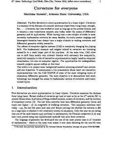
Fig. 1. Various curves and corresponding discrete traces (shaded areas). (a) Distinct planar curves may share a common discrete trace, (b) a small orientation change is undiscernible, (c) a comer and a bend of high curvature have identical traces, (d) two orientation changes in close proximity and a smooth bend have similar discrete traces.

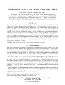
shown that it is not sufficient to infer only the trace of a curve, but that tangent and curvature fields must be inferred as well. Again, we formulate these discretely. The tangent and curvature fields embody the smoothness assumptions, and act as further constraints on the inverse sampling problem. Thus, the tangent and curvature estimates provide a local “model” of the curve in a neighborhood around each putative trace point. To illustrate the different orders of constraint, Fig. 2 depicts a discrete trace to which continuous curves have been fitted. Given points in the discrete trace Fig. 2(a), a discrete orientation constraint (through the discrete tangent field) is added in Fig. 2(b), and then the combined orientation and curvature constraints (through the discrete tangent and curvature fields) are in Fig. 2(c). Observe that the curves in Fig. 2(c) and (b) satisfy the positional constraint in Fig. 2(a); that is, they all pass through the indicated positions. Similarly, the curve in Fig. 2(c) satisfies the tangent constraint in Fig. 2(b), but not vice versa. Finally, the curve in Fig. 2(c) satisfies a curvature constraint (depicted as short arcs of osculating circles), and it is also the smoothest curve satisfying these combined constraints. Thus, additional (smoothness) constraints limit the space of possible curves; what is required for our problem is to provide sufficient constraints so that there is a unique curve which satisfies them. The problem is then well posed. We now start to concentrate on the trace inference problem, and begin our search for constraints with a review of differential geometry. More global smoothness constraints limiting the full space of possible curves will, of course, influence the analysis. These will also be discussed in appropriate places. C. Overview of Differential Geometry It is useful to review a few elementary notions of differential geometry [7] to establish the context in which the smoothness constraints will be formulated. The review will be centered on curves in the plane, although generalizations to higher dimensional curves exist.

825

Fig. 2. Three curves fitted to a given discrete trace: (a) positional constraint only, one fit among a large family of curves with a broad spectrum of behavior; (b) position and orientation constraint, the family of curves is more constrained; (c) position, orientation and curvature constraints combined with a smoothness criterion, the family of solutions is reduced to a single curve. Observe that the curve in (c) satisfies the orientation (tangent) constraint and that both curves (c) and (b) satisfy the positional constraint (a). But the curve in (a) does not satisfy the tangent (b) or curvature (c) constraints.

Let I be an interval in one-dimensional Euclidian space E’. A curve C is defined as a continuous mapping x: I -+ E2 from the interval to the plane where 44

= (KIWI X2(t))?

(2.6)

with t E I being a parameter running along the curve, and xl, x2 continuous functions oft. The curve is said to have order of continuity k, denoted Ck, if all derivatives up to and including the kth derivative of X, and x2 are continuous. Taking the first derivative with respect to t everywhere along C, we obtain the tangents x’(t) = (4(t),

G(t))

(2.7)

where the vectors x’(t) have bases at (x,(t), x2(t)). Their magnitudes can be interpreted as the velocity of a particle following the curve. A curve may be reparameterized in terms of its arc length s, equivalent to a particle traveling at constant unit velocity along the curve. In this case, the tangent vectors are unit length vectors x’(s) = (4(s), x;(s))

(2.8)

where s = f(t) is a reparameterization of the curve, and IIX’II = 1. The interesting aspect of the tangent is its orientation. The geometric interpretation of the tangent to a curve is depicted in Fig. 3(a). Letting P be a point on a curve, and A a neighboring point, the tangent T at P is the limit of the line AP as A approaches P along the curve. The tangent yields the orientation of a curve at a point. Taking the second derivative with respect to s everywhere along C, we obtain

x”(S) = (x;‘(s), .6(s))

(2.9)

where the vector x”(s) is normal to the vector x’(s), and the magnitude of x”(s) is called the curvature of C. Curvature is a measure of the rate of change of orientation per unit arc length. The geometric interpretation for the

826

IEEE TRANSACTIONS ON PATTERN ANALYSIS AND MACHINE INTELLIGENCE,

c

d (a)

dL-l (b)

Fig. 3. (a) Tangent T is the limit of segment z

Cc) as A approaches P along

C. (b) The curvature K of C at P is the limit of the ratio cr/ 1G 1 as A and B approach P independently along C. (c) The osculating circle 0 at P is the limit of the circle that passes through A, P, and B as A and B approach P independently along C.

curvature is depicted in Fig. 3(b). Let P be a point on a curve, T the tangent at that point, and A a neighboring point on the curve. Let (Y denote the angle between the line AP and T, and 1%?I the arc length between A and B. The curvature K at P is the limit of the ratio CY/IB] as A approaches P along the curve. Related to this interpretation of curvature is the osculating circle. Referring to Fig. 3(c), let A, P, and B be three neighboring points on a curve, and let 0 be a circle through these points. As A and B independently approach P along the curve, the circle 0 converges towards a limit, whose radius is precisely the inverse of the curvature K at P. D. Derivatives Through Curvature Consistency Although third and higher order derivatives can be defined for curves, practical considerations dictate that the process must stop somewhere. Our position is that the trace, tangent and curvature fields provide the local basis for inferring global curves, and are necessary for placing discontinuities, corners, or breakpoints. Moreover, as we shall show, these are all the derivatives that can be computed stably, and even then only when they are approximated coarsely, in this first stage of analysis of the image. Qualitatively for people, interesting events along curves consist only of abrupt changes of orientation and curvature, local maxima of curvature, and inflection points (i.e., zero crossings of curvature) [I], [13], [17], and [9]. These are the places that a human observer is most likely to choose to segment long curves into shorter ones. Higher order discontinuities such as discontinuities in curvature variation do not seem to matter. Between the selected corner points, curves simply appear to be smooth. Although this argument for limiting the number of derivatives considered is informal and based on human perception, any machine vision system will have to confront this issue as well. While any number of derivatives can be defined, only a finite (and, in fact, small) number of them can actually be computed. Evolution, presumably, has settled upon an optimal number. In terms of differential geometry, then, the visual system would appear to perceive curves as being piecewiseC”, with segmentation occurring at discontinuities in the first and (certain) second derivatives of the curves. In the sequel, we shall show that curvature consistency-a necessary relationship between discrete estimates of curva-

VOL. II. NO. 8. AUGUST 1989

ture along a smooth curve-amounts to a bound on the third derivative, i.e., on the curvature variation. Higher order discontinuities are implicitly smoothed over and ignored. There is a numerical reason for limiting the analysis to curvature variation as well. Quantization can be modeled as the addition of “noise” [21], and each derivative numerically amplifies this noise. It is well known that the numerical stability of computing higher-order derivatives is poor. Although we shall come back to this point later in this paper, for now suffice it to note that some number of derivatives are necessary to control smoothness and to signal discontinuities, and we shall take that number to be 3. Furthermore, real care must be used in computing them. E. Tangent and Curvature Fields So far, we have thought about curves intrinsically, i.e., as given functions x (s ) of an arc-length parameter s. However, since this is primarily the object we are after, and not given, it is necessary to formulate some of our algorithms extrinsically in terms of the Euclidian space in which the curves are embedded. Consider a retinotopic restriction of the plane E2 to finite domain D C E2. We shall be interested in 2 fields on D, one which is a mapping that associates tangent vectors x’(s) to points in D, and the other which associates curvatures x”(s). We refer to these fields as tangent and curvature fields, respectively. The fields form the basis of our representation for (a local description of) curves. Thus, those points in the trace of a curve will have unit tangents mapped to them, while others will have null tangents. Discontinuities will have multiple tangents. F. Discrete Representation of Trace, Tangent, and Curvature Since our problem begins in the discrete domain, we choose a representation for curves based on their traces, with associated tangent fields and curvature fields. These latter fields are represented discretely as well, to reflect the fact that curve inference consists of a two-stage process. In this first step, the goal is to estimate the trace, tangent, and curvature fields finely enough so that discontinuities can be placed, but coarsely enough so that overwhelmingly restrictive assumptions are not made. The compromise solution, then, is with discrete tangent and curvature fields, which serve as inequality bounds on which the next, global stage can be based [37]. The discrete trace of a curve consists of a set of points in the discrete plane. The discrete tangent field is formed by finding, for each point of the discrete trace, the quantized orientation of the curve as it runs through that point. It thus consists of a set of unit tangents to curves, characterized by their position and orientation. Hence, letting 19~denote the discrete orientation of the tangent at a particular position, X = 1, * * * , m, the actual orientation 0* lies in the interval (2.10)

PARENT AND ZUCKER: TRACE INFERENCE, CURVATURE

CONSISTENCY, AND CURVE DETECTION

The discrete curvature field is similarly formed by associating to each unit tangent the quantized curvature at that point. It is desirable to have a uniform representation for all points in the discrete plane, capable among other things of distinguishing between trace points and nontrace points. If, for example, the orientation of a curve is allowed to have one of 8 values, i.e., the orientation is quantized to multiples of E = 7r/8, each point of the discrete plane could be associated with a vector of 8 elements, each one a predicate true or false according to whether or not a curve passes through that point with approximately that (quantized) orientation. Alternatively, the true or false predicates could be replaced by real numbers in the interval [ 0, 1 ] where the extremes assert presence or absence of a curve with absolute certainty, while intermediate values represent less certain assertions. Thus, for curve points, there is at least one element of the certainty vector with a value near 1, while for noncurve points, all elements are near 0. Some points may have more than one near-l value, e.g. curve crossings, and orientation discontinuities. ’ The following notation is used for the certainty of tangent X at position (xi, yi):

827

IV. TRACE INFERENCE AND ORIENTATION SELECTION The goal of the first stage of our curve inference process is the recovery of local information. Clearly, this must

include the recovery of trace points. If the curve were known, then trace points could be separated from other image structure simply by calculating them. But the curve is not known, so we are forced to estimate the structure of the curve in the neighborhood of each putative trace point. As we shall show, coarse estimates of the tangent and curvatures provide sufficient local information about the curve. These estimates provide a partial local model for the curve sufficient to gather evidence about individual trace points from their neighbors. Two terms used above-local and coarse-warrant further expansion because they are related in a fundamental way. Observe that, when searching for a book in the library, one first searches through broad categories before finely scanning the exact titles. Analogously, curve recovery is facilitated by first obtaining a rough-or coarseestimate of its structure to guide subsequent analyses. The need for a local analysis follows for similar reasons, since few (if any) assumptions can be made a priori about the global structure of the curve. Moreover, given the presence of noise from both sensors and quantization, such a coarse, local analysis becomes necessary; imaging trying to exactly estimate the tangent of a contour from an image to three decimal places without strict a priori assumptions, such as the straightness of the sides of a block [3]. Seeking higher order approximations suffers the same problems as well. Similar arguments could be made in detail about the tangents and curvatures. If the curve were known, then these could be computed exactly. But since it is not, then they must be estimated as well. There is something of a hierarchy of information here, with the (estimated) tangents supplying constraints on the positions of nearby (estimated) trace points, with the (estimated) curvatures supplying constraints on the (estimated) tangents and their (estimated) locations, and, finally, with curvature consistency relationships supplying constraints on (estimated) curvatures. Moreover, this hierarchy holds for quantization as well. Observe that a quantization of the image plane imposes a quantization on orientation which is necessarily coarser than the quantization on position. Next, the quantizations of position and orientation impose a still coarser quantization on curvature, and so on for higher order properties, with change in curvature being the highest one can go. This, then, provides the rationale in principle for restricting our local models to coarse changes in curvature: one simply cannot compute the necessarily coarser higher order properties. We now develop these constraints in detail, based on quantizations of the differential geometry already described. In the end we will have obtained an inference procedure for estimating (quantized) trace, tangent, and curvature fields such that a particular functional with terms through curvature variation is minimized.

‘More formally, at orientation discontinuities we represent the tangents obtained through the limiting process in both directions, or the so-called Zariski tangent space [ 111. These are important for the second, global stage of curve inference; see [37].

, A. The Two Steps of Stage 1 The Stage 1 inference procedure consists of two distinct steps, a measurement step and an interpretation step. The

pi(X)

for i = 1, * * * , n X = 1, * * * , m.

(2.11)

assuming an image with n pixels and m possible orientations of tangents at each pixel. pi(h) = 1 indicates that tangent X is definitely associated with (xi, vi). With each orientation vector element pi(X) is associated a single discrete measure of curvature, Ki( h). It becomes part of the discrete curvature field when the corresponding tangent is part of the discrete tangent field. For a generalization in which there is a set of discrete curvatures associated with each discrete trace position, see 1371. III. CURVE INFERENCE AS A TWO-STAGE PROCEDURE Sufficient background material has now been developed to specify the two stages involved in inferring a curve. Stage 1: Trace Inference and Orientation Selection Taking an image as input, infer the discrete trace, tangent, and curvature fields subject to quantization and maximal curvature constraints. 2) Curve Synthesis Taking the discrete trace, tangent, and curvature fields as input, locate discontinuities and find integral curves running through the fields subject to discontinuity and smoothness constraints. Stage 2, curve synthesis, will be treated in a subsequent paper [37]. We now concentrate on Stage 1.

828

IEEE

TRANSACTIONS

ON

PATTERN

functional minimization and tangent field inference are accomplished in the second step. In particular, Step I: Measurement Convolution of linear operators against the image to obtain initial tangent estimates at each position and for each (quantized) orientation. Step 2: Interpretation Selection of a subset of the tangents signaled in Step 1 according to the functional minimization procedure to be defined. Classically, of course, the linear operators amount to “line detectors’’ [27], although our selection procedure is much more complicated than simply taking the “strongest” convolutions. Rather, it amounts to selecting those “strong” convolutions that are strongly supported by-or consistent with-the other convolutions in their neighborhood according to the estimated local curve model. We now discuss the two steps in turn. 1) Step I: Initial Tangent Estimates: The requirement for the first step is a set of operators that estimate the presence of a tangent at each position in the image. Since discretely the tangent can be viewed as a short, straight line segment, templates tuned to this structure are the obvious candidates. Such templates amount, of course, to so-called “line detectors” [27], [33], and we use the following one (see Fig. 4): G(x, y) = B’(x)

* exp (-~‘/a;)

(4.1.a)

with LSF(x) = exp (-.x2/o:)

- B exp (-x2/u;)

+ C exp (-x2/0:).

(4.1.b)

The classical rationale for choosing such operators is clear: they are template representations of short, straight line segments. The Gaussian kernels have the attractive property that they smooth over intensity variations along the tangent direction, but sharpen them in the orthogonal direction [36]. Such operators resemble the receptive fields of so-called simple-cells in primate visual cortex [ 141, and hence are also attractive from a biological point of view. 2) Step 2: Interpreting the Initial Tangent Estimates: Classical treatments of curve detection also involve two steps, the first of which is very similar to the one just described. But the second step-interpretation of the operator convolutions-is usually much simpler than the scheme that we shall be describing. Since the operator templates match high-contrast straight lines so well, it is often assumed that simply selecting the strongest convolutions is sufficient for obtaining a local representation of the contour (what we are calling a tangent field). But this is not the case for any pattern other than widely spaced, straight lines. Curvature, comers, and nearby contours all affect the convolutions, and all are sufficient to invalidate the maximum convolution selection strategy [33], [35]. A richer model for curves is clearly needed. From the differential geometry reviewed in Section II,

ANALYSIS

AND

MACHINE

INTELLIGENCE,

VOL.

II.

NO.

8. AUGUST

1989

Fig. 4. The initial convolutions are performed with ihis “line detector” operator, which is a difference of three Gaussians in the x direction, multiplied by a single Gaussian in the y direction.

it is clear that our model must at least include curvature. Recall that, in the neighborhood of each point, the osculating circle is a substantially better approximation to the curve than the tangent (Fig. 3). We shall later argue that curvature is also a high-enough approximation to separate closely spaced curves, so that incorrect convolutions that cover distinct curves can be properly interpreted. Therefore, we shall focus on curvature, and shall begin to derive an estimation procedure based on (a quantized version of) it. Our goal, briefly stated, is to minimize the curvature variation at each point by maximizing circularity. V.

POSITION,

ORIENTATION,

AND

CURVATURE

CONSTRAINTS

In this section, we shall first establish the neighborhood circularity measure in terms of a pairwise relation between (estimated) tangent elements, called cocircularity, which determines an orientation constraint. Introducing the maximum curvature constraint that arises from grid quantization is then straightforward. Second, it will be shown that the orientation constraint is not sufficient and that interaction between neighbors should be mediated by a curvature consistency constraint. This constraint can be applied provided local estimates of curvature are available. It will be shown that these estimates can be obtained by partitioning neighborhoods into regions called curvature classes, and that tangent estimates can be obtained by propagating support through these regions. Consistency of curvature is achieved by comparison of the curvature classes. Finally, a level of constraint is required to achieve the high localization accuracy which is characteristic of curvilinear patterns in images. This positional constraint is a form of lateral maxima selection whereby a pixel-wide region is determined to be part of the curve. It is required because support for tangent elements may occur over a relatively wide area near curves, whereas the discrete trace of a curve is composed only of the set of pixels through which the curve actually passes. This level of constraint thus insures the correctness of the trace inference. A. Cocircularity The standard approach to estimating curvature is to fit a polynomial to a collection of points, and then to differ-

829

PARENT AND ZUCKER: TRACE INFERENCE, CURVATURE CONSISTENCY, AND CURVE DETECTION

entiate the polynomial twice [24]. This, however, amplifies noise, and hence is unusable in our quantized context. We shall present a different scheme, in which the information contained in tangent estimates provides the basis for curvature estimates through the cocircularity relationship. I) Dejnition: The relation of cocircularity applies to distinct tangents to a circle [see Fig. 5(a)]. A property of this spatial configuration is that the tangents form angles of equal magnitude, but of opposite sign, with the line joining the points of tangency [see Fig. 5(b)]. Thus, abstraction can be made of the circle, and the symmetry of the configuration can be retained as the characteristic of cocircularity. Note that when the radius of the circle becomes infinite, we obtain a special case of cocircularity, colinearity. Cocircularity is therefore a function of both the orientations and the positions of the tangents. Dejnition: Two unit tangents X and X’ are cocircular, denoted XXX’ iff there exists a circle to which they are both tangent. Cocircularity is a kind of symmetry relation between tangents, and bears some relationship to the way in which [4] define a local symmetry. But our discretization and use of the notion differs substantially from theirs. 2) Cocircularity in the Discrete Case: When position and orientation are quantized, tangent pairs are seldom exactly cocircular. The small perturbations introduced by quantization must somehow be taken into account. To do this, we begin by allowing the position of the tangents to be anywhere within the circle of radius l/2 pixel centered at the pixel. Likewise, we let their orientation vary within a neighborhood of size E, for orientations quantized to multiples of E. The tangent pair is thus cocircular if there, exists at least one assignment of the position and orientation variables for which cocircularity as defined above is true. Let (xi, yi) and (Xj, Yj) be the coordinates of nodes i andj, and let (x, y) be an arbitrary point within the circle of radius l/2 centered at (Xi) yi), and (x’ , y’ ) a point in a circular neighborhood of (xj, yj); let X and X’ be unit tangents at these locations and &, and t+,, be their respective orientations; let 19be an orientation in an e-neighborhood of f3,,,and 8’ an orientation in an e-neighborhood of oh’(see Fig. 6). The orientation of the line joining the centers of the pixels is given by 13, = arctan (Ay/Ax)

(5.1)

where Ax = Xj - xi and Ay = yj - vi. We wish to determine the minimum and maximum values that may be taken by 0,, the orientation of the line joining the tangents as (x, y ) and (x’ , y’ ) are allowed to vary within their circular neighborhoods. As in Fig. 7, the extrema coincide with the two intersecting tangents common to the circular neighborhoods. In the case of circles of equal radii, it can be shown that the angle between the common tangent and the line joining their centers is

y---J

‘p

(b) “‘k

a Fig. 5. In (a), unit tangents A and B are both tangent to the same circle, therefore A is cocircular to B (denoted AXE). This condition is geometrically equivalent to that depicted in (b) where 01 = -0.

Fig. 6. Two unit tangents X and A’ with respective orientations Oh, Xx, whose positions are restricted to the circle of radius l/2 centered at the pixel positions (x,, y,), (x,, y,); the line with orientation fl,, joining the centers of the pixels; the line with orientation 8, joining the tangents.

Fig. 7. The interval for the orientation 0, of the line joining two curve tangents located in circles of radius l/2 centered at (x,, y,) and (x,, yj) is ( Oij - (Y, tlij + (Y) where Oij is the orientation of the line joining the centers of the circles, and (Y depends on the distance d, separating them. The sine of (Y is l/2 divided by the distance from 0 to (x,, y,), which is d,/2, hence Q = arcsin (l/d,,).

given by c11= arcsin (l/&).

(5.2) Let the function I’(p, y) designate the interior angle between a pair of lines with orientations p and y, as in Fig. 8. Let the sign of this function be the same as the direction in which the first line must rotate in order to close the interior angle and coincide with the second, that is, positive for counterclockwise and negative for clockwise rotations. The formal definition of this function, assuming that 0 I /3 5 7r and 0 I y 5 7r, is the following:

w,

Y) =

Y - P,

if 1-r - P( I T;

r-P-r,

if4

< y - fi I a;

i

L Y-0+x,

if --T I y - /3 < -t. (5.3)

830

IEEE TRANSACTIONS ON PATTERN ANALYSIS AND MACHINE INTELLIGENCE,

Fig. 8. The interior angle function r (0, y) is the interior angle between a pair of lines with orientations 0 and y. The sign of this function is determined by the direction in which the first line must rotate in order to close the interior angle.

Turning back to Fig. 6 and recalling the geometrical definition of cocircularity , we find that the tangents at (xi, Yi) and (Xj, yj) are cocircular if the interior angle between the first tangent and the line joining the tangents is the same as that between the latter line and the second tangent. Formally, X”, h’ iff w,

4) = rut,

0’1,

(5.4)

for some e, E (e, - (Y, 8, + CY), 8 E (e, - e/2, ex + E/2), 8’ E (e,. - e/2, Ox, + e/2). This condition is clearly equivalent to Jr(eA, e,) - r(e,,

e,.)/ < E + 2a.

(5.5)

Condition (5.5) is a discrete cocircularity condition; it is either true or false. A continuous version of this condition can be implemented by measuring the closeness to cocircularity, and we refer to this measure as a cocircularity coefficient. Departure from exact cocircularity occurs by rotation of one of the tangents, which suggests that a function of the difference in orientation between a tangent and the cocircular tangent in the same position could be used as a measure of cocircularity. The cocircularity coefficient then consists of a real number between 0 and 1, where 0 means not cocircular, 1 means cocircular, and values close to 1 are interpreted as nearly cocircular. Generally, the coefficient is 1 for a certain range of orientations of tangents at the neighboring node, because of built-in quantization noise tolerance in (5.5). Denote this range by [ emin, &,,,I. We let the magnitude of the coefficient fall off monotonically outside this range (see Fig. 9). Thus the cocircularity coefficients cii ( X, X’) are given by 1,

if 1w,

e,) - v,,

e,.) (

< E + 20;

c&L, A’) = max(l

-

+h,

otherwise

-

emI,

Cmin)>

(5.6)

VOL. II, NO. 8, AUGUST 1989

Fig. 9. Cocircularity coefficient c,, (A, A’) as a function of orientation !$. of neighboring tangent. The length of the interval [ 8,,,, e,,,] is e + 201 [see condition (5.5)].

where 8, is the extreme of the range [ emin, &,,,I closest to &,‘, and 7 is the absolute value of the slope of the dropoff region, assuming a linear decrease. Because of the grid and tangent quantization, it is necessary to consider tangents distributed in a neighborhood around each image point. If only the 3 by 3 immediate neighborhoods were considered, then the angular quantization of 0, would be much too severe. The cocircularity coefficient so defined can be measured for all neighboring tangents in a neighborhood of a given size, and the set of these measures forms the neighborhood support set. 3) Maximum Curvature Constraint: In order to introduce the maximum curvature constraint [recall Fig. 1(c)], a measure of the radius of curvature implied by a pair of tangents is required. Letting sij ( X) denote the implied radius, we use ‘&)

= 2 sin 1r (e,, e,) 1

(5.7)

as its measure. The maximum curvature constraint implies that cij(X, X’) = 0 whenever 6,(X)

< Pmin+ (5.8)

Fig. 10(a) shows the set of neighbors cocircular to a tangent with a vertical orientation for a neighborhood diameter of 15 with the maximum curvature constraint applied. B. Cocircularity Support We are now in a position to estimate how well a particular (estimated) tangent is supported by other (estimated) tangents in its neighborhood. Recall that the first measurement stage consisted in convolutions against “line detectors” (Section III). Letting oh, denote the orientation of the operator at position i = (xi, y;), X = 1, * * * , m, the normalized convolutions ( p;(X), i = 1, * * * , n, X = 1, *** ) m } , 0 I pi ( X) 5 1, provide an initial estimate of the confidence in tangent X at position i. Note, for a long straight line of orientation oh* passing through i, that pi (X*) will be maximal at that position, and that pi(X) will drop off from pi (h*) according to the orientation tuning curve for the operator. But when the curve does not consist of long straight lines, pi(X) can follow a more complex distribution at each point i. Therefore, the circularity measure must be

PARENT

AND

ZUCKER:

TRACE

INFERENCE,

CURVATURE

CONSISTENCY,

AND

Cd)

I

CURVE

831

DETECTION

/-” (b)

(a) L,, y’

(cl

:,, ,,

,:,,_I

,;\ I 5

.I:

Ay- L \

(a) \.

(b)

Fig. 11. In (a), AXB and A and B are tangent to the same curve. In (b), however, the spatial configuration of A and B is the same as in (a), but they are tangent to distinct curves.

:‘I

(e)

(0

w

04

Fig. 10. A diameter 15 neighborhood (a), partitioned into 7 curvature classes for the vertical orientation (b)-(h). These 7 distinct curvature classes thus represent the coarse quantization of curvature or, equivalently, the discrete number of equivalence classes obtained by projecting continuous osculating circles onto our discrete representation. The choice of 7 classes was empirical and based on the observations that 1) it is fine enough to support curve and discontinuity localization, but 2) coarse enough to be reliably computable. (a) bears some resemblance to the consistency operators for curve enhancement developed in [ 121.

evaluated over a local neighborhood around i and must depend on the entire distribution of possible tangents at each point. W e take a linear weighted sum to indicate the cocircularity support for a unit tangent X at position i S;(A)

= j*,

,$,

rij(x3

x')Pj(x'>

where rij( X, X’) = cv( X, h’), the cocircularity coefficient. Clearly, those tangents lying along a curve should have maximal support. More remains to be done before this is guaranteed, however, because linear averaging schemes such as this have the potential to smooth across different but nearby (within the given neighborhood) curves. A more sophisticated formulation as a closestpoint problem is under way [ 161. C. Curvature Classes Consider a small neighborhood of an image containing many curves. W ithin this neighborhood, many tangent pairs are mutually cocircular, with some cocircular pairs belonging in fact to distinct curves. More specifically, given three tangents A, B, and C in such a neighborhood and given that A,-B and AXC, it does not follow necessarily that BXC. In particular, the interpretation of A remains ambiguous when B ,“C: does A belong to the curve going through A and B, or to the one through A and C? One way to decide the situation is to partition the neighborhood support set about A into sufficiently narrow curvature classes Xk (A ), k = 1, * . * , K as in Fig. lO(b)(h). Each curvature class consists of all the osculating circles whose radius is between the limits for that class or, equivalently, whose curvature is within certain limits. Thus, if A x B, A x C, and B, C belong to the same curvature class Xk (A) with respect to A, it may be concluded that BXC. Two benefits accrue from the use of partitioning. First, it imposes n-wise consistency of tangents within curvature classes at a low cost in complexity. The tangent support function can be modified to take advantage of the

partition, by measuring support independently by curvature class, and by selecting the highest as the final tangent support. The support of tangent X at node i is thus given bY n m s;(X) = max C C $(A, X’) (5.9) k=I,Kj=l X’=l pj(A')

where the coefficient ri(X, X’) is the product of the cocircularity coefficient cij (X, X’) and a partitioning function if&in

5

otherwise;

&j(X)

5

Pk,,,;

(5.10)

for given curvature class limits phi” and piax. The second benefit is that a discrete estimate of curvature K~ (X) is obtained by correspondence with the curvature class that maximizes the support function. W ith this estimate, it is be possible to introduce a further constraint on the selection of neighboring tangents for local support. This constraint is examined in the next section. First note, however, that these discrete curvature estimates have been obtained without the numerical problems inherent in standard, spline-fitting techniques. In technical terms, relations between tangents in a curvature class amount to connections in fiber bundles; see [28]. D. Consistency of Curvatures One kind of ambiguity persists even after partitioning into curvature classes. Consider, for example, Fig. 1 l(a) and (b). In Fig. 1 l(a), tangents A and B are cocircular and they are tangent to the same curve. In Fig. 11(b) however, tangents A and B occur in the same spatial configuration as in (a), yet they are tangent to distinct curves. Should the tangents A and B mutually support each other in (b)? If not, how can configurations (a) and (b) be told apart? The solution to this problem requires comparison of local curvature class estimates. The orientation of a tangent and the local curvature class estimate together determine a region about the position of the tangent where a curve is most likely to exist. In Fig. 12, B ,VA, therefore B belongs to at least one of the curvature classes of A. But in Fig. 12(a), the local curvature class estimate at B does not include A as a member. The curvatures are said to be inconsistent and this condition precludes mutual support of A and B. Fig. 12(b) depicts a situation where curvatures are consistent with the interpretation that a curve passes through A and B. Note that in this case we have

832

IEEE TRANSACTIONS ON PATTERN ANALYSIS AND MACHINE INTELLIGENCE,

VOL. II, NO. 8. AUGUST 1989

have f 1,

iffp,(X)

> p,(h’),

Vh’

E {X - 1, X, X + l}, and (4

Fig. 12. In (a), AXB but the estimated curvature at B is inconsistent with the interpretation of a curve through A and B. In (b) however, mutual support is possible because the curvatures are consistent. It is this condition that involves a coarse estimate of change-in-curvature, and naturally provides a mechanism for locating (orientation) discontinuities.

both A E X,(B) and B E X,,(A) for some k and k’ (not necessarily equal). Letting Ci!‘( X, X’) denote the predicate variable for curvature consistency, i.e.,

cy’(x,

A’) =

Pi(A) > PrW), VA’ E {X - 1, X, X + l}, and

(b)

1,

if curvature class k of X at i is consistent with estimated curvature class k’ of h’ at j ;

0,

otherwise;

W+(h) = {

PiCx> > Pi(x’>,

E {A - 1, h + l}; ( 0,

r-y’< A, A’) = cij( A, A’) Ki(X, A’) CF’( X, A’),

where pl( X’) and p,( X’) denote the certainties of the left and right interpolated certainties for tangent X’. As an alternative to interpolated certainties, one could just as well perform a strict comparison against a set of neighboring certainties determined by the orientation of the certainty under test. Comparison sets can be defined in such a way that the selection process is stable. More formally, 1, Q(A)

E. Lateral Maxima In this section, we address the problem of inferring the trace of a curve from the certainties associated with the tangents in a tangent network during our procedure. The objective is to extract a pixel-wide region about a curve, i.e., to prevent thickening of the curve in the discrete trace. The method is based on comparisons between certainties in a small neighborhood, with selection of the tangents with highest certainty, i.e., the lateral maxima. 1) Techniques for Extracting Lateral Maxima: The rationale for inference by lateral maximum selection is the observation that the support function exhibits a characteristic maximum at the precise location of a curve, and decreases gradually on either side of this location. Lateral maxima selection is, in principle, a simple technique, but its implementation on a discrete grid requires careful consideration. The most obvious problem is that, on an orthogonal grid, only those tangents whose orientation is parallel to a grid axis have lateral neighbors with which to compare. For other orientations, interpolated values for lateral neighbors must be used, rather than the neighbor closest to the ideal position. A straightforward linear interpolation based on a plane fitted to the three nearest neighbors is quite sufficient. A tangent h at (x, y ) is therefore a lateral maximum if its certainty is maximal among all tangents in the 3 by 3 neighborhood in positionorientation space. Letting rn; ( X) denote the predicate variable for a lateral maximum for orientation h at node i, we

=

iffpi(X)

> pj(X’), VA’ E {X - 1, X9

A + l}, VjENk, L 0,

(5.12)

which is a function of curvature as well as orientation and position.

otherwise; (5.13)

(5.11) we obtain a new coefficient

vx’

(5.14)

otherwise;

where the neighbor set Nx is a predefined set depending on the orientation X. The lateral maximum property of neighboring tangents can be used as an additional constraint in the support function. Since only those tangents in the neighborhood that are lateral maxima are compatible with a curve interpretation (observe that the initial convolutions drop off with lateral displacement from the curve), the support function should be correspondingly restricted. Thus, we obtain a new expression for the support of a tangent Si(X)

= max C C $‘(A, k= ],K j= 1 A’= I

X’)pj(X’)

mj(X').

(5.15) The net effect of this constraint is to further narrow the region near curves where tangents receive support. VI. INFERRING

TANGENT

FIELDS

BY

MAXIMIZING

SUPPORT

Since the expression (5.15) for the support of a tangent should be maximized at each position, a natural choice for a global functional is the average local support

Qualitatively, the pi(X) indicate which tangents and positions are chosen, and the si( X) indicate how mutually consistent they are through the quantized geometrical constructs just developed. That is, the Si(h) codes the local model for the curve in the neighborhood of position i

PARENT

AND

ZUCKER:

TRACE

INFERENCE,

CURVATURE

CONSISTENCY.

and the tangent h. In particular, as the positional quantization Ai -+ 0, orientation quantization Ax + 0, and the curvature classes approach the actual curvature, si (X) --t 1 for all tangents along the (smooth) curve, and s;(X) + 0 elsewhere. Relaxation labeling is a procedure for maximizing expressions such as (6.1) [ 151, and in the following section, we review the relaxation labeling procedure and tailor it to this application. A. Overview of Relaxation Labeling Relaxation labeling is an iterative procedure applied over a network of nodes. Associated with each node is a set of labels, and associated with each label is a measure of confidence, or certainty. Let there be II nodes and, for the sake of simplicity, a unique set of m labels at each node. Further, let pi(X) denote the confidence of label X at node i. The values of the p;(h) are restricted to the interval [ 0, 11, and are subject to the added constraint that at each node i At, PiCAl = l

fori = 1, * 9 * , n.

(6.2)

In vector notation, this constraint can be written as p’; * 1 = 1 where 1 is the m dimensional vector of l’s ( 1, 1, . . . , 1). The degree of compatibility between a label and its neighborhood can be measured by what is known as the label’s support, which is a function of other label certainties in the neighborhood and their compatibility (pairwise) with the label being supported. The constraints between labels are represented by a matrix of compatibilities, rii( h, h’), which serve to embody the problem-dependent knowledge. In this notation, ru( X, X’) denotes the compatibility between label h’ associated with nodej and label X associated with node i. Relaxation labeling is the process of achieving consistency. Hummel and Zucker [ 151 defined consistency in variational terms; they also proved that, for symmetric compatibilities, consistent states of the relaxation network maximized functionals of the form A ( p) in (6.1). Such maxima are achieved iteratively: beginning with an initial labeling { pp( X) }, the iteration d”(A)

= f(d(Q

d(V)

(6.3) continues until convergence. Hummel and Zucker [15] develop a general scheme for the iteration (6.3) utilizing the Mohammed [19] projection operator. However, the efficiency of this scheme can be improved substantially for this application; see [22] and Appendix A. B. The Relaxation Graph The original approach [32] to representing curves in a relaxation graph used m orientations of tangents to a curve at each node, plus the no-line label, with certainties subject to condition f?l+1 Az, p;(X) = 1, for i = 1, * . . , n. (6.4)

AND

CURVt

DElhCTlVN

833

According to this convention, a labeling is consistent and certain only if at most one orientation is chosen by the relaxation process. However, curve intersections and corners require that multiple orientations be chosen at certain nodes. Our solution is to have not one but many superimposed relaxation graphs, one for each label h = 1, * * * , m. W e shall refer to this collection as a network of relaxation graphs. Each node of graph X requires 2 labels: h and noline. Network interactions are permitted between the relaxation graphs through the compatibility matrix. Note that the certainty vector at each node of each graph consists of two components with unit sum. Clearly, nothing is gained by representing both components of the vector explicitly, one of the components being simply the complement of the other. Similar savings can be achieved in the compatibility matrix by eliminating the no-line label completely. The advantages of this network of relaxation graphs are twofold. First, multiple labels at a position (as arise when curves cross or bifurcate) need not compete with one another. Rather, they are supported by the context provided by their own relaxation graph. Second, since each label only competes against a null label, only positive information needs to be represented explicitly. This is analogous to the biological situation in which firing rate varies with confidence, and can formally be obtained as follows. Consider the contribution of node j to the support of the two labels (0 and 1) at node i. Letting rl , = r,j( 1, 1 ), rlo = rij ( 1, 0)) etc., andpj = pi ( 1 ), we obtain, from (A.2.a), r,0(1

-

Pj>

+

rl$j

(6.5)

S;(O) = cdl

-

Pj>

+ ro#j.

(6.6)

S;(l) =

Assuming that roe = r,,, ro, = rIo = -rll, reduced to Sf( 1) = 2 ’ r,,(pj

- 1)

Si(0) = -Si(l)

the above are

(6.7) (6.8)

where both expressions are void of terms related to label 0. Hence, for this special case (and many similar ones where all compatibilities are functions of a single one), it is possible to reduce the complexity of the relaxation graph and the compatibility matrix.2 The assumptions about the compatibilities are not unreasonable when label 0 is interpreted as no-line. This result shows that if certain labels are left out and only the compatibilities between the remaining labels are specified, the system is equivalent to another one where all the labels and compatibilities are specified. Thus, truncation of the graph and compatibility matrix does not violate relaxation labeling theory. The result is extensible to systems of more than two labels. ‘A compatibility each pair of labels.

matrix is the matrix of compatibility

coefficients

for

834

IEEE

TRANSACTIONS

O N PATTERN

C. Complete Relaxation Model To summarize, a sketch of the complete relaxation model as it will be used in the trace inference process is as follows. Network: m graphs of n nodes, one for each orientation. The labels represent tangents with orientations quantized to multiples of E. The “no-line” label is not explicitly represented. The m labels at node i have independent certaintiespi E [0, 11. Si( X) of label X at node Support Function: The support i is a normalized function of the sum of the products of neighboring label certainties by appropriately chosen compatibility coefficients, as in (5.15). Update Formula: Each pi ( h) is updated as though in a two-label graph, with the other label interpreted as “noline” and having complementary support, i.e., -s,(h). pi(X) is updated in such a way as to converge asymptotically to 1 when excited, and to 0 when inhibited. D. Normalization Details Two details remain, but they are central to successful implementations. First, the support functions must be normalized to account for arc-length effects, and second, they have to be mapped into a common interval so that values are comparable across positions. We discuss each of these normalizations in turn. I) Extent of Neighborhood Support: The unit tangent support function has so far been described in terms of cocircularity coefficients, but nothing has been said about the shape or extent of the neighborhood over which tangents interact. We could assume a circular neighborhood shape, determined by the neighborhood diameter and the maximum curvature constraint. However, this circular shape is not ideal because arcs of different curvature have distinct intraneighborhood lengths, implying a bias of the support function towards longer arcs. In order to make the support of a tangent to a curve independent of the particular curvature, the extent of the neighborhood is adjusted so that arcs of circles with all curvatures have the same intraneighborhood length. Letting R denote the maximum arc length distance of interaction between unit tangents, the curve describing the boundary of the equilength region is given by

in polar coordinate form. Fig. 13 depicts such a neighborhood, with the minimum radius of curvature rmin = 1 /Knm constraint applied. The neighborhood is thus composed of all unit tangents whose arc length distance 8, (h) I R. The estimated arc length distance can be obtained from the estimated radius of curvature &(X) with a,(x)

= 2iij(M

(m,

e,> I.

(6.10)

Letting Eli denote the neighborhood extent predicate, we have

ANALYSIS

AND

MACHINE

INTELLIGENCE,

VOL.

II.

NO.

8, AUGUST

1989

Fig. 13. An equilength neighborhood for the vertical orientation with 7 curvature classes. All arcs of circle vertically tangent to the center of the neighborhood have the same length.

1,

if a,(x)

I R;

(6.11) otherwise. 0, 2) Intrapixel Length Correction: Next, we consider the intrapixel length correction to the compatibility coefficients. This is necessary in order to ensure that the process is isotropic. A straight line of a given length intersects a different number of pixels of a digital grid depending on its orientation. For example, diagonal lines intersect fewer pixels than lines of the same length at any other orientation, while the lines parallel to a grid axis intersect the most. Unless a compensation is introduced, the process will therefore “prefer” orthogonal orientations to diagonal ones. A simple normalization coefficient is given by Eij =

Jz

(6.12) A’ where ox, is the angular difference between Ox! and the nearest grid axis. With this compensation, we obtain the final expression for the compatibility coefficients by multiplying the expression of (5.12) by l( X’), giving w>

$‘(A,

= 2

A’) = cij(X, X’) EtiK$(X, X’) $‘(A,

A’) 1(X’) (6.13)

where Cij( X, X’) is the cocircularity coefficient, 8$(X, X’) is the curvature class partitioning function, and Cf’( X, X’) is the curvature consistency predicate. 3) Normalization of the Support Function: The support function obtained previously is

(6.14) but its range must be normalized before use. For a given neighborhood radius, one can compute the integral of the local compatibilities given that a single curve (assume a straight line) traverses the entire neighborhood in the proper orientation. Denote this integral by S max. This sum determines the maximum support that a

PARENT AND ZUCKER: TRACE INFERENCE. CURVATURE CONSISTENCY. AND CURVE DETECTION

label can obtain from its neighborhood, and the sum varies according to the radius of the neighborhood. This is the maximum support that can be achieved. The minimum acceptable support for a label depends both on geometry and noise. First, the process should be stable near the end of a curve; that is, the curve should neither grow nor shrink during relaxation. Second, a threshold can be established according to the response of the initial operator convolutions in the presence of pure noise. Now, consider the pixel at the end of a low contrast line. The operator response, which is sensitive to contrast, will be rather low at that point, while the integral of the compatibilities would be approximately s,,, /2 (the curve traverses only half the neighborhood), times the average certainty of the labels on the curve. Assuming a minimum contrast criterion Pminwe fix the minimum acceptable support of a label as Smin

=

Pmin $rnax ___

(6.15)

2

With this choice of smin, relative stability at end-lines is insured for a wide range of initial contrasts. If, on the other hand, the initial contrast of a curve is below the minimum, then that curve will gradually shorten until it disappears. The label support is normalized by mapping the interval [ smm3smax ] linearly into the interval [ 0, 11. The required normalized support, S;(X), is therefore S,(X) =

s;(x> s max

-

Smin Smin

(6.16) ’

It can readily be seen that this expression is equal to 1 when the raw support si( X) equals the maximum support smaxwhile the numerator vanishes if the raw support equals the minimum acceptable support, srnin. Of course, anything less for the raw support leads to a negative normalized support. The normalization of the support occurs before the projection of the support vector at a node onto the positive quadrant; see Appendix A. This completes the discussion of the technical issues related to the implementation of a discrete trace inference process within a relaxation labeling computational framework. We turn our attention now to the results of the trace inference process over various kinds of images. VII. EXPERIMENTS In discussing the experiments performed with the trace inference process described in the preceding sections, we will go from simple to complex. Thus, in the first part of this section, we discuss experiments based on artificial images designed to evaluate specific features of the process, such as sensitivity to curvature, and robustness in the presence of noise. At the same time, the trace inference process is compared to other procedures to extract curves from images, in the presence of large amounts of noise. Further experiments based on real images, such as biomedical imagery, satellite imagery, and fingerprints, are discussed in the second part of this section.

835

Fig. 14. Trace inference process on concentric circles after 2 iterations. The resulting tangent field (short segments) and curvature field (arrows pointing to center of curvature) are superimposed on the image (filled pixels). The assigned tangent and curvature fields are perfect everywhere except at a few locations were quantization affects the local structure of the cutve more severely. These errors would disappear using a larger neighborhood size.

Implementations were done on a DEC VAX 1 l/780 running VMS. Although the run times for the experiments were very long (up to 12 hours), the algorithm is totally parallel and can readily be implemented in parallel hardware. A. Artijicial Images 1) Sensitivity to Curvature: The first experiment is designed to evaluate sensitivity to curvature. Referring to Fig. 14, the image is composed of 4 concentric circles whose radii were chosen to match individual curvature classes. The following parameters are used for the initial operators (see (4.1) for the parametetized form of the operator) : 01 = 1.14 a2 = 1.8 u3 = 2.28

cry = 3.6

B = 1.266 C = 0.5.

(7.1) A neighborhood diameter of 15 pixels is used, with 7 curvature classes determined by the following radius limits (in pixels): radius limits: 2.7, 4.2, 7.2, 21.0 (7.2) The result displayed in Fig. 14 is after 2 iterations, with step size 1, and using a supporting threshold Smin= 0.5. In these displays, tangents are indicated by short line segments, and curvatures by vectors pointing toward the center of the osculating circle. The magnitude of the curvature vector is proportional to the radius of curvature. 2) Sensitivity to Noise: The next experiment is designed to evaluate the effect of noise on the trace inference process. The image consists of a single hand-drawn curve on a uniform background, featuring a sharp orientation discontinuity and varying curvature. The experiment is performed independently for two neighborhood sizes, 15 and 25 pixels, respectively, and for each size there are 5 noise levels: S/N = 00, 1.?,0.9,0.6, and 0.45. The noise added to the image has uniform distribution U(0, A), where A is the peak-to-peak amplitude of the noise. Given that the curve has constant intensity Z, over a background of con-

836

IEEE

Neighborhood

size 15

TRANSACTIONS

Neighborhood

O N PATTERN

ANALYSIS

AND

MACHINE

INTELLIGENCE,

VOL.

II.

NO.

8. AUGUST

1989

size 25

(a)

(b)

Cc)

Cd)

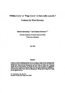
Fig. 16. A comparison of different methods for detecting curves: (a) intensities thresholded to include most of the curve points, resulting in many noncurve points being selected; (b) thresholded lateral maxima, equivalent to the 0th iteration of the trace inference process; again, only a low threshold allows all curve points to be selected, at the cost of including some noncurve points; (c) previous Parent and Zucker method, based on comparison of expected versus observed operator responses; this method is not curvature-based, and depends only on the immediate 3 by 3 neighborhood for support, hence, the noise sensitivity; (d) trace inference process, same as previous figure for neighborhood size 25 and S/N = 0.45. It clearly illustrates the advantage of using curvature information.

Fig. 15. Trace inference on an image consisting of a single curve, using two neighborhood sizes, and with the addition of various amounts of noise, to obtain S/N ratios of 03, 1.8, 0.9, 0.6, and 0.45. After two iterations, only those tangents with certainties above 0.5 are displayed. The smaller neighborhood size results in fairly stable inference down to S/N = 0.9, while the larger neighborhood size remains quite stable for S/N down to 0.45 where the curve is nearly imperceptible at close range.

stant intensity Zb, the S/N ratio is obtained by ,qN

=

Izc -

A

Ibl

’

(7.3)

Both experiments use 7 curvature classes, and the radius limits for each size are as follows: size 15 radius limits: 2.7, 4.2, 7.2, 21.0 size 25 radius limits: 4.5, 7.0, 12.0, 35.0.

(7.4) The initial convolutions are with operators whose size is adjusted to the respective neighborhood sizes. For the smaller neighborhood size, the parameters are those in (7. l), and for the larger one, the parameters are as follows: 01 = 1.9 a2 = 3.0 u3 = 3.8 uY = 6.0 B = 1.266 C = 0.5.

(7.5) The results displayed in Fig. 15 are after 2 iterations, using a supporting threshold Smin= 0.5. The performance of the trace inference process in the presence of noise is very satisfactory, especially for the larger neighborhood size. To emphasize these results, a comparison between various other methods for selecting curves is displayed in Fig. 16. These are based on the same curve as in Fig. 15, at S/N = 0.45, the noisiest case.

In Fig. 16(a), an optimal intensity threshold is chosen, interactively, so that most of the curve points are selected, but this results in too many noncurve points being selected at the same time. Significant additional processing would be required to remove these noise points. In Fig. 16(b), a threshold is applied to the lateral maxima based on an initial operator size of 25, as for the large neighborhood of Fig. 15. This result is in fact the 0th iteration of the trace inference process, and hence resembles a process of selecting the maximal response at each position. Again, to obtain all curve points, a low threshold must be chosen, resulting in too many noncurve points, and significant post-processing would be required. In Fig. 16(c), the result displayed comes from an earlier attempt to formulate an inference process [34] in which consistency is achieved through comparison of expected versus observed operator responses. This method is corner-sensitive, and slightly curvature-sensitive, and thus represents an improvement over an earlier method using only tangent information [32], the result of which is not displayed here. The effective neighborhood diameter for this experiment is 3. Thus, this procedure has only slight curvature sensitivity, and does not have a built-in noise removal capability for short low-contrast segments as in the trace inference process. It is no surprise then, that this method also degrades rapidly in the presence of noise. Finally, in Fig. 16(d), the result for the largest neighborhood at S/N = 0.45 from Fig. 15 is reproduced. Comparison to the rest of the figures clearly indicates the importance of curvature information. B. Natural Images The preceding experiments on artificial images showed that the curvature information helped the trace inference

PARENT AND ZUCKER. TRACE INFERENCE. CURVATURE CONSISTENCY. AND CURVE DETECTION

(a)

(a)

Fig. 17. (a) An angiogram, or radiograph of blood vessels in the brain, and (b) the result of 2 iterations of the trace inference process over the image of an angiogram.

(b)

Fig. 19. The result of 2 iterations of the trace inference image of a fingerprint

over the

neighborhood size, 11 pixels in diameter, was chosen. However, the initial convolutions were performed with the same operator as for the angiogram experiment, i.e., with parameters as in (7.1). Again, 2 iterations of the process were used. The display threshold for the tangents is set to 0.3, a low value because the image itself had low contrast. Observe how the tangent field follows the contours exactly, and how end points and bifurcations are handled implicitly. Stability over neighborhood size is also illustrated, since almost no “clumping” of tangents arises (Fig. 19). (a)

(b)

Fig. 18. A satellite image of a forest with logging roads, and (b) the result of 2 iterations of the trace inference process, using a neighborhood size of 25, a step size of 1 .O, and displayed at a confidence threshold of 0.6. The curvature vectors are omitted for the sake of clarity.

process to find curves in controlled situations. The main interest of the procedure, however, lies in its application to finding curves in real images, such as satellite images, biomedical images, and fingerprints. In this section, three experiments based on such images will be described. I) Angiogrum: The first experiment takes a biomedical image as its input, an angiogram, or a radiograph of blood vessels in the brain. It is a good example of an image with many curves, all of which have varying curvature, with many curve crossings at various angles. The image is first convolved with operator parameters as given in (7.1). The neighborhood size is 15, the number of iterations is 2, with a step size of 1. All tangents with a certainty of at least 0.5 are displayed in Fig. 17, however, the curvature vectors are omitted for the sake of clarity. 2) Satellite Image-Logging Roads in Forest: The second natural image experiment is based on a satellite image of forest terrain in which logging roads are visible as light, elongated streaks, on a slightly darker background. The experiment is performed using a size 25 neighborhood, with parameters for the initial convolution as in (7.5), and radius limits as defined in (7.4) for size 25. The inference process is run for two iterations, with a step size of 1 .O. The result displayed in Fig. 18 is thresholded at a confidence level of 0.6. 3) Fingerprinr: The final experiment involves a fingerprint image. For computational efficiency, a smaller

VIII. SUMMARY AND CONCLUSIONS Information about the exact structure of curves is lost when they are projected into quantized images. Hence, curve detection is an inferential process, utilizing both image information and other constraints. We formulate the curve inference process as two distinct stages, in which local information is first recovered so that it can guide the global stage. In this paper we concentrated on the recovery of local information, and demonstrated that it could be accomplished both in theory and in practice. Images contain information not directly about curves, but rather about their traces, or the set of quantized image positions through which the curve passes. But these traces are not uniquely specified; they must be separated from other image structure. Therefore, the first stage of curve inference must include trace inference, and the development of an approach to this occupied most of this paper. Inherent in trace inference is a chicken-and-egg problem. If the functional form of the curve were known, then the trace could simply be calculated. But since it is not, most of our effort went into developing an estimation procedure sufficiently powerful to provide a model for the curve in the neighborhood of each possible trace point. The model for curves included the tangent and curvature at each point, and it is this model that guided trace inferences. The result was what we called a tangent field, or a representation of the trace, tangent, and curvatures suitably quantized. Since it is the high-frequency microstructure of curves that is lost through quantization, it is natural to employ smoothness constraints while estimating them. We derived such an estimation procedure by examining how dis-

838

IEEE TRANSACTIONS ON PATTERN ANALYSIS AND MACHINE INTELLIGENCE.

cretization and quantization effect their differential-geometric definitions. The result was a functional with terms through curvature variation which could be maximized to guide trace inference. It appears that functionals through curvature variation are necessary to properly separate the influences of nearby curves, yet are sufficient to place discontinuities. The computation of curvature is notoriously sensitive to noise. To avoid these problems, we introduced an altemate method for coarsely estimating it, based on average values of tangent estimates within spatial neighborhoods called curvature classes. Computing the tangent field was the overall goal of the first stage of curve inference, and we demonstrated that curvature and curvature consistency (or limits on curvature variation) can be utilized advantageously. Several examples illustrated that the trace could be recovered reliably, and that the information in the tangent field certainly provides a rich, stable foundation for global curve inference. RADIAL

APPENDIX

A

UPDATE

RULE

PROJECTION

FOR

RELAXATION

LABELING

Consistency is the state of a relaxation network where the certainties of all labels are in agreement with their support, that is, labels with high certainties have large support while those with low certainties obtain little support. This notion can be stated as follows. Dejinition: A labeling is consistent if and only if the labeling assignment vector matches the normalized support vector at every node, that is, fii = I T.

fori=

?; * 1

1, a** ,~t.

(A.1)

In [23], an efficient update rule is described that achieves consistency as defined above. This method utilizes radial projection instead of normal projection to avoid the complexities incurred at the boundaries of the labeling space. This Appendix summarizes the [23] paper to some extent; for further details and the relationship to classical relaxation, please consult it. Three steps are required to obtain updated labeling assignments using the radial projection method. Given the initial measures of confidence, pp( X), and the compatibility coefficients, rU ( h, X’), the first step is accumulating the support evidence for each label n $(A>

= jz,

m Az,

rii(L

A’)

pi(h’).

(A.2.a)

The second step is a projection, if required, of the support vector at a node onto the boundary of the positive quadrant, to avoid labeling outside the valid assignment space SF = min s:(h)

(A.2.b)

X=l,m Sk(A) $(A)

= sf;(X)

-

,-;

if Sf I 0; otherwise.

(A.2.c)

VOL. II. NO. 8. AUGUST 1989

Finally, the third step is the radial projection method as such. It consists, for each node i, of the scaled vector sum pf + s’“”

(A.2.d) 1’ I This rule amounts to taking, from the current assignment, a step in the direction of the nearest consistent assignment. The magnitude of this step is governed by the quantity p’:+’

=

&I =

1 +

s’?k.

s’,?” . 1 1 + ?T”* 1

(A.2.e)

where it is known that 0 I (Ys < 1. The rate of convergence CX~can be modified by scaling the support vector ?” uniformly throughout the network by any positive constant, called the step size. REFERENCES F. Attneave, Applications of Informafion Theory to Psychology: A Summary OfBasic Concepts, Methods, and Results. New York: Holt. Rinehart and Winston, i959. ]2] H. G. Barrow and J. M. Tenenbaum, “Interpreting line drawings as three-dimensional surfaces,” Arrijicial Intell., vol. 17, pp. 75-116, 1981. [3] T. 0. Binford, “Inferring surfaces from images,” Artijcial Inrell., vol. 17, pp. 205-244, 1981. ]4] M. Brady and H. Asada, “Smoothed local symmetries and their implementation,” Robot. Res., vol. pp. 37-61, 1984. [5] L. S. Davis and Freeman, “Comer detection in chain codes,” IEEE Trans. Pattern Anal. Machine Intell., 1977. [6] L. S. Davis and A. Rosenfeld, “Cooperating processes for low-level vision: A survey,” ArtiJicial Intell., vol. 17, pp. 245263, 1981. En[71 M. P. do Carmo, Differential Geometry of Curves and Surfaces. glewood Cliffs, NJ: Prentice-Hall, 1976. [8] 0. Faugeras and M. Berthod, “Scene labeling, An optimization approach, ” in Proc. IEEE Conf: Pattern Recognition Image Proc., Chicago, IL, 1979, pp. 318-326. [9] M. A. Fischler and R. C. Bolles, “Perceptual organization and curve Proc. 1983 Image Understanding Workshop, 1983. partitioning,” [lo] S. Geman and D. Geman, “Stochastic relaxation, Gibbs distributions, and the Bayesian restoration of images,” IEEE Trans. Parfern Anal. Machine Intell., vol. PAMI-6, pp. 721-741, 1986. New York: Springer Verlag, [11] R. Hartshome, Algebraic Geometry. 1972. [12] M. Hedlund, G. H. Granlund, and H. Knutsson, “A consistency operation for line and curve enhancement,” in Proc. Patrern Recognition Image Proc. Conf., 1982, pp. 93-96. [13] D. D. Hoffman and W. A. Richards, “Parts of recognition,” in From Pixels ro Predicares, A. Pentland, Ed. Norwood, NJ: Ablex, 1986. [14] D. Hubel and T. Wiesel, “Functional architecture of macaque monkey visual cortex,” Proc. Royal Sot (London), vol. B198, pp. l-59, 1977. 1151 R. Hummel and S. W. Zucker, “On the foundations of relaxation labeling processes, ” IEEE Trans. Pattern Anal. Machine Intell., vol. PAMI-5, pp. 267-287, 1983. selection to optical flow: ]16] L. Iverson and S. W. Zucker, “Orientation A computational perspective,” Proc. IEEE Workshop Cornput. Vision, Miami, FL, 1987. [17] J. Koenderink and A. Doom, “The shape of smooth objects and the way contours end,” Perception, vol. 11, pp. 129-137, 1982. “An application of heuristic search methods to edge and 1181~;n~~~~~;ection ” Commun. Assoc. Comput. Mach., vol. 19, pp. ’ 11-83. 1976. [19] J. L. Mohammed, R. Hummel, and S. W. Zucker, “A gradient projection algorithm for relaxation methods,” IEEE Trans. Pattern Anal. Machine Intell., vol. PAMI-5, pp. 330-332, 1983. [20] U. Montanari, “On the optimal detection of curves in noisy pictures,” Commun. Assoc. Comput. Mach., vol. 14, pp. 335-345, 1971. [21] A. Papoulis, Probability, Random Variables, and Stochastic Processes. New York: McGraw-Hill, 1965. [22] P. Parent and S. W. Zucker, “Radial projection: An efficient update [l]

PARENT AND ZUCKER: TRACE INFERENCE. CURVATURE CONSISTENCY. AND CURVE DETECTION rule for relaxation labeling,” Comput. Vision Robotics Lab. Tech. Rep. TR-85-15R, McGill Univ., 1985. “Radial projection: An efficient update rule for relaxation la1231 beling,” IEEE Trans. Pattern Anal. Machine Intell., to be published. Rock~241 T. Pavlidis, Algorithms for Graphics and Image Processing. ville, MD: Computer Science, 1982. t251 S. Peleg and A. Rosenfeld. “Determining compatibility coefficients for curve enhancement relaxation processes,” IEEE Trans. Syst., Man, Cybern., vol. SMC-8, pp. 548-555, 1978. VW A. Rosenfeld, R. Hummel, and S. W. Zucker, “Scene labeling by relaxation operations,” IEEE Trans. Syst., Man, Cybern., vol. SAC6, pp. 420-433, 1976. New York: t271 A. Rosenfeld and A. Kak, Digital Picture Processing. Academic, 1976. P. Sander and S. W. Zucker, “Inferring differential structure from V81 3D images: Smooth cross sections of fiber bundles,” McGill Res. Cent. Intell. Machines Tech. Rep. TR-CIM-88-6, McGill Univ., Montreal, P.Q., Canada, 1988. visual information from multiple ~291 D. Terzopoulos, “Integrating sources,” in From Pixels to Predicates, A. Pentland, Ed. Norwood, NJ: Ablex, 1986. [301 D. Waltz, “Understanding line drawings of scenes with shadows,” of Computer Vision, P. H. Winston, Ed. in The Psychology New York: McGraw-Hill, 1975, pp. 19-91. [311 A. P. Witkin, “Recovering surface shape and orientation from texture,” ArtiJcial Intell., vol. 17, pp. 17-45, 1981. ~321 S. W. Zucker, R. Hummel, and A. Rosenfeld, “An application of relaxation labeling to line and curve enhancement,” IEEE Trans. Comput., vol. 26, pp. 394-403, and pp. 92-929, 1977. [331 S. W. Zucker, “Early orientation selection and grouping: Evidence for type I and type II processes,” Comput. Vision Robot. Lab. Tech. Rep. TR-82-8R, McGill Univ., 1982. operators and optimal [34] S. W. Zucker and P. Parent, “Multiple-size curve finding,” in Multiresolution Image Processing and Analysis, A. Rosenfeld, Ed. New York: Springer-Verlag, 1984. [35] S. W. Zucker, “Early orientation selection: Tangent fields and the Image dimensionality of their support,” Comput. Vision, Graphics, Processing, 1985.

839

[36] S. W. Zucker and R. Hummel, “Receptive fields and the representation of visual information,” Human Neurobiology, vol. 5, pp. 121128, 1986. [37] S. W. Zucker, C. David, A. Dobbins, and L. Iverson, “The organization of curve detection: Coarse tangent fields and fine spline COVerings,” McGill Res. Cent. Intell. Machines Tech. Rep. TR-CIM88-17, McGill Univ., Montreal, P.Q., Canada, 1988; also in Proc. 2nd ICCV, Tarpon Springs, FL. Pierre Parent received the Bachelor’s degree in economics from Universite de Montreal in 1975, and the Master’s degree in electrical engineering from McGill University in 1987. He managed the computer facilities of the Computer Vision and Robotics Laboratory and the VLSI Laboratory at McGill University for many years. He began an MBA degree at McGill University in 1987 and, having obtained the Schulich Scholarship for Entrepreneurship in 1988, graduated in 1989. He is currently pursuing a business career in the area of hardware applications of computer vision and VLSI.

Steven W. Zucker (S’71-M’75-SM’86-F’88) is a Professor of Electrical Engineering at McGill University, and the Codirector of the Computer Vision and Robotics Laboratory in the McGill Research Center for Intelligent Machines. He was elected a Senior Fellow of the Canadian Institute for Advanced Research. Dr. Zucker obtained his education at CamegieMellon University in Pittsburgh and at Drexel University in Philadelphia, and was a post-doctoral Research Fellow in Computer Science at the University of Maryland, College Park. He has authored or co-authored more than 130 papers on computational vision, image processing, artificial intelligence, biological perception, and robotics.