gent visual surveillance, teleconference and real-time animation from live motion ... With eigenface approach, a face image can be represented as a linear sum ...
Tracking and Recognition of Face Sequences S.Gong†, A.Psarrou‡, I.Katsoulis†, P.Palavouzis† † Department of Computer Science, Queen Mary and Westfield College, University of London, Mile End Road, London E1 4NS, UK ‡ School of Computer Science, University of Westminster, New Cavendish Street, London W1M 8JS, UK
Abstract In this work, we address the issue of encoding and recognition of face sequences that arise from continuous head movement. We detect and track a moving head before segmenting face images from on-line camera inputs. We measure temporal changes in the pattern vectors of eigenface projections of successive image frames of a face sequence and introduce the concept of “temporal signature” of a face class. We exploit two different supervised learning algorithms with feedforward and partially recurrent neural networks to learn possible temporal signatures. We discuss our experimental results and draw conclusions.
1
Problem Statement
Face recognition is important for the interpretation of facial expressions in applications such as intelligent man-machine interface and communication, intelligent visual surveillance, teleconference and real-time animation from live motion images. There have been many computer models proposed for machine-based recognition of face images [21, 17, 4]. Among them, the eigenface approach, initially introduced by Sirovich and Kirby [19, 9] for face image coding and then adopted by Turk and Pentland [21] for classification, extracts principal local and global hidden “face stimuli” that are significant in recognition. The distinctive features of this method are: the eigenvectors reflect the statistical properties of face images they represent; they capture more global “signatures” of the faces and therefore, more tolerant and immune to local variations. Because face recognition is commonly subject to a wide range of changes in viewing angle and facial hair as well as to partial occlusion and blurring, the eigenface method is computationally more robust [12] and biologically more plausible than other template matching techniques that are based on the detection of visible local facial features and the representation of face models by geometric measures of such features, for example the location and size of eyes, nose and mouth as well as their distance. Eigenfaces also provide an attractive mechanism for the transmission of coded image sequences through networks. However, there is a fundamental problem with the existing eigenface models. Current eigenface models only recognize single face images that have been taken from a strict narrow view angle, most commonly a frontal view. This substantially limits its robustness and ef1
Face subspace for the frontal view (0 degree)
Face subspace for 45 degree view
Face subspace for profile view (+/- 90 degree)
Figure 1: The face space and sub-spaces associated with different view angles. fectiveness [15]. For example, two face images of the same face class (i.e. an individual) are more likely to be identified with different classes if the difference in viewpoint is large. Temporal information of time sequences provides important constraints in recognition. We introduce the concept of “temporal signature” in face recognition. Instead of recognizing single “snapshots” of a face, a sequence of face movement is taken into account for a coherent interpretation. In the rest of this paper, we briefly describe in section 2 the computation of pattern vectors following the notion of Turk and Pentland [21]. In section 3, we address the issue of head tracking and segmentation of face images. We describe two different types of neural networks that are designed to learn temporal characteristics in face sequences in section 4. We draw our conclusions in section 5.
2
Face Representation
With eigenface approach, a face image can be represented as a linear sum of a set of eigenfaces. These eigenfaces are normalized eigenvectors which are the principal components of a “face space” and they characterize distinctive variations in facial appearance. In general, for a set of M face images that have an unified size N , where N = m×n and (m, n) are the width and height of an image, a N -dimensional face space can be defined where face images are points in this hyperspace (see figure 1).
2.1
From Eigenfaces to Pattern Vectors
Given a set of face images Γ1 , Γ2 , . . . , ΓM , an average image can be computed as: M
Ψ=
1 X Γi M
(1)
i=1
2
and a new set Φ1 , Φ2 , . . . , ΦM is given by Φi = Γi − Ψ. This simply translates the original face images by Ψ in the face space 1 . Then the principal components of the new face space given by Φi are the eigenvectors of the following covariance matrix: M
C=
1 X T Φi ΦT i = AA M i=1
where A = [Φ1 Φ2 . . . ΦM ] and C are N×N matrices. For a typical image size 2 , computing the N eigenvectors of C is computationally hard. However, since the number of the face images is much smaller than the dimension of the face space (M ≪ N ), there only exists M − 1 nontrivial eigenvectors with the remaining ones associated with negative or zero eigenvalues. Now, if we consider Vi to be the eigenvectors of matrix AT A whilst AT A is only a M × M matrix, i.e. (AT A)Vi = λi Vi where λi are the eigenvalues, then A(AT A)Vi = A(λi Vi ), which means (AAT )(AVi ) = λi (AVi ) and AVi are the eigenvectors of C = AAT . Therefore, the eigenvectors of C are given by: i v1 .. . M i X = v Ui = AVi = [Φ1 . . . Φk . . . ΦM ] (2) vki Φk k . k=1 .. i vM where (i = 1, . . . , M − 1) and vki is the kth element of Vi . Then the eigenfaces are the normalized eigenvectors with image pixel values. For a given set of eigenvectors Uk , a face image Γ can be projected onto the eigenvectors by: ωk =
UT k (Γ − Ψ) λk
k = 1, . . . , M ′
(3)
where Ψ is the average face image given by equation (1), λk are the eigenvalues and M ′ ≤ M − 1 3 . Now, we have a weight distribution vector Ω = [ω1 ω2 . . . ωM′ ] known as the pattern vector of Γ. A face image can therefore be represented by its pattern vector and the first M ′ eigenfaces of the face space. If we regard the eigenfaces as the basis set of the face space, then ωk ∈ (−1, 0) ∪ (0, 1). Now, for all the face images in the given set that belong to the same face class (i.e. an individual), one computes an average pattern vector Ω. This can be regarded as the “signature” of that face class. For a new face image, one calculates the Euclidian distance ε between its pattern vector and the Ω of a known face class ε =k Ω − Ω k. Then, this face image can be identified with the known face class if ε falls within a given threshold. 1 For calculating eigenvectors, Φ are computationally more stable since their values are i much smaller compared with those of Γi . 2 For an image size of 256×256, the dimension of the face space N is 65536. 3 With M ′ < M − 1, the representation is approximate.
3
So far we have assumed that face images are taken from a very similar view. In reality, face images appear from different views (e.g. face image frames arise from continuous head movements). With the method described, two face images of the same class but with large view difference are more likely to be associated with two different classes. This is because that eigenfaces do not explicitly register any three-dimensional facial structure and images are not differentiated in any way if they are taken from different view angles. For face images with large view difference, the number of eigenfaces required has to be large enough in order to cope with the vast face space due to the number of samples needed for individual view angles of each face class. Our experiments show that for just 4 face classes, if 5 common views are taken into account, 30 face images are used to represent one view of each class, to calculate only the first 120 eigenfaces of the face space (having 600 − 1 meaningful eigenfaces) required over 18 hours of computation on a typical workstation plus over 100MB of memory space. This is computationally very expensive, even just for 4 people. One obvious solution to the problem is to divide the face space into a set of sub-spaces where each sub-space is associated with a typical view angle. However, with such an approach, it is not obvious how to associate an unknown face image to any of the face sub-spaces unless an exhausted projection of the given face image into all sub-spaces is carried out. This again requires expensive computation. In the following, however, we first address the issue of getting face images.
3
Segmentation of Face Images
In order to encode face images by eigenfaces, it is necessary to obtain face images in the same size from the camera input. If large areas in the images that are used to form a face space contain background rather than face information, the extracted eigenfaces would say more about the statistical properties of the background than that of the faces. Camera inputs need to be processed in order to locate, track and segment only the face images.
3.1
Bootstrapping the Region of Interest
The first step of the computation requires the detection of a “region of interest” (ROI), assuming only one head movement in a given scene being of our interest. This bootstrapping process is based on the information of motion detected in the images. Accurate and consistent estimation of visual motion is hugely time consuming [5]. For real-time processing, we apply two filtering techniques that only compute partial motion and detect possible temporal change respectively. We show that such information is sufficient for the purpose of locating the ROI. 3.1.1
Detection and estimation of movement
With a spatio-temporal Gaussian filter: 2 2 2 2 a G(x, y, t) = u( )3/2 exp−a(x +y +u t ) π
4
where u is a time scaling factor and a gives the width of the filter as wm = √ 2σ 2, a symmetric second order temporal edge operator is given by [1]:
√2 a
=
1 ∂2 )G(x, y, t) (4) u2 ∂t2 By convolving image frames I(x, y, t) of a temporal sequence with this operator m(x, y, t)⊗I(x, y, t), spatio-temporal zero-crossings can be located in the output images S(x, y, t). For avoiding the computational complex of a three-dimensional convolution, the above operator can be approximated by three one-dimensional operations in x, y and t independently [1, 13]. As a result, the temporal filtering takes place over 8 image frames in time, i.e. it can only start from the eighth frame of a sequence. With the output S(x, y, t), one can calculate the normal components of visual motion along the spatio-temporal zero-crossings. For accuracy, however, the convolution window size wm requires to be ≥ 8 so that the output image S(x, y, t) is linear over a 3×3×3 neighbourhood. That means the computation of the normal motion at any given time requires at least 3 successive image frames. Therefore, it starts at the 10th frame of a sequence. Now, let Sijk = S(x + i, y + j, ut + k) be in a three-dimensional cubic neighbourhood of a zero-crossing point (x, y, t) in S, then a least-squares fitting of Sijk to a linear polynomial fijk = f0 + fx i + fy j + fz k gives: P P P 1 1 1 fx = 18 (5) ijk iSijk , fy = 18 ijk jSijk , ft = 18 ijk kSijk m(x, y, t) = −(∇2 +
As a result, the spatio-temporal gradient of S at (x, y, t) estimates the normal visual motion as: −ufz (fx , fy ) (6) (x˙ ⊥ , y˙ ⊥ ) = 2 fx + fy2
Figure 2 shows the effect of applying such a filter to image sequences. It is necessary to point out, though, that this spatio-temporal filter measures continuous motion that lasts for more than eight image frames. When the head movement is rapid and head position changes significantly in less than eight frames, the computed visual motion field gives a poor indication of head positions. In order to address rapid head movements, an additional fast motion detector is introduced. This process does not measure any visual motion but it copes well with large temporal changes in fewer image frames. By subtracting two spatially Gaussian smoothed 4 successive image frames in a sequence, we obtain images that only contain regions of temporal change (see figure 3). This operation can be sensitive to sudden changes in lighting conditions and the output of a subtraction is subjected to a threshold that is often heuristic. 3.1.2
Initialization of ROI
In the outputs of the motion detectors described above, one marks the locations of movement. The boundaries of moving regions can then be grouped and segmented. With a single ROI, this can be easily done by determining the extreme 4 Palavouzis
gives detailed discussions on not using spatio-temporally smoothed images [13].
5
Figure 2: The spatio-temporal zero-crossings of images from two different sequences and the corresponding normal visual motion. location of moving pixels. For multiple regions of interest, Gong and Buxton [7] demonstrated an adaptive segmentation algorithm based on Bayesian belief networks. After finding out the approximate boundaries of a ROI, an elliptic active contour is initialized with its centre, major and minor axes being determined by the distance between the left and right, the upper and lower boundaries. There are a number of advantages in using an active ellipse over the more traditional active snakes based on splines. Studies by Torr et. al. [20] show that whilst they share a common feature for small number of parameters, ellipse does not suffer from two common drawbacks of other snakes, i.e. part of a snake often gets left behind so the curve straddles front and back of the contour it tries to follow, and a snake sometimes crosses itself or folds and partially collapses onto itself. Figure 4 shows two examples of initializing a ROI by ellipse.
3.2
Head Tracking
Fitting an ellipse with the initialization process in every frame is unreliable and inconsistent since individual points in visual motion are often fragmented in time. Robust tracking requires continuous updating of the parameters of the elliptic contour. We apply Kalman filters [8] to model the dynamics of these parameters and to predict future movement of an ellipse in order to provide more accurate estimation of its position in time. A Kalman filter is a recursive, linear optimal filter for state estimation in dynamic systems. A system state can be a single variable or a vector that describes the characteristics of the system. For an active ellipse, it has four temporal parameters (ignore the orientation for the 6
Figure 3: Top: Two successive image frames of a sequence. Bottom left: The result of subtracting the spatio-temporal filtered two frames. It shows that information about the movement of the head (i.e. turning from left to right) is evident whilst the location of the head in the current frame is unclear. Bottom right: The subtraction of spatially filtered image frames which gives more accurate indication of the head position. time being). Assuming that the position of an ellipse is uncorrelated with the length of its axes, a dynamic system can be used to describe both coordinates of the centre of an ellipse with its position, velocity and acceleration. For the x coordinate (similar for y), an update condition is given by: x 1 ∆t ∆t2 /2 x 0 1 x˙ ∆t x˙ + 1/2 vacc + 0 vpos = 0 1 x ¨ k+1 0 0 1 x ¨ k 1 0 where vacc and vpos are noise covariances for assumptions about constant acceleration and position estimation, and a measurement model is given by zk+1 = xk+1 + w, where xk+1 is the actual state vector at time tk+1 and w is a noise covariance vector for measurement errors. zk+1 is the observation vector at time tk+1 . For updating the major and minor axes of an ellipse, we use a different dynamic system where its state is the length of one of the axes. The update condition for the major axis (similar for the minor axis) is: lk+1 = lk + vl where vl is the noise measure for constant length assumption and the measurement model is zk+1 = lk+1 + u, where u is an error measure in the measurement of length. Setting parameters is rather crucial for a Kalman filter to perform. The noise and error covariances are usually determined by experiments. Our experiments 7
Figure 4: Initialization of an active elliptic contour based on the detection of movement in image frames. show that the appropriate values for vacc and vpos are between (1.5, 2.0) whilst w = [2, 0.5, 0.2], vl = 10 and u = 4. Palavouzis gives a detailed description and analysis on tuning the Kalman filters [13]. We take the average of the normal optic flow field given by equation (6) as an estimation for the ellipse’s velocity and the temporal difference between velocities of successive frames as the estimation for acceleration. Consequently, the Kalman filters are initialized at the 11th frame and start to update at the 12th frame of an image sequence. The results of a tracking process can be seen in figure 5.
Figure 5: Two snap shots of the head tracking process.
4
Recognition of Face Sequences
Temporal information in time sequence provides important constraints in recognition [6, 18]. To divide a face space in time not only overcomes the ambiguity in mapping a target image with its corresponding sub-space since they share a time reference, but also takes the continuity in the temporal changes of face images into account. Instead of recognizing any single “snapshot” of a face, a temporal sequence of face movement is taken for recognition. In the following, we give details about our neural network approach for dividing a face space in time. 8
Images per sequence
1 2 1 2 Sequences
. . .
N
First face subspace
. . .
M
x
y
z
x
y
z
x,y,z: All the first, second , Mth (respectively to x,y,z) images of individuals 1,2,...,L
Individual
x
y
.. .. ..
z
Second face subspace
. . .
x
y
z
x
y
z
Mth face subspace
Individual
x
1
y
L
z
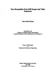
Figure 6: M temporal face sub-spaces for a feedforward neural network classifier.
4.1
A Feedforward Neural Network Classifier
A key factor that needs to be considered when applying feedforward neural networks (FFNNs) is the training time required to learn efficient information from a set of training patterns. Past experiments in applying FFNNs to learn face images [10] have shown to be computationally expensive because mapping face images to neural networks requires vast amount of training in order to capture meaningful information. However, the eigenface representation enables the pattern vectors to be used in place of images. This hugely reduces the dimension of patterns involved in training. We divide the face-space of face sequences into a set of temporal sub-spaces that correspond to groups of possible face orientations associated with time. We capture a set of sequences of continuous head movements in front of a stationary camera. Each sequence has M image frames. Every image frame in a sequence contributes to one group of possible head orientations associated with a given time (see figure 6). We compute the pattern vectors of each sub-space and train independently M FFNNs in order to encode the sequences with M subspaces. During training, pattern vectors of a specific time instance are applied to a network and are classified into different face classes. During recognition, the network is presented with a pattern vector of a face image from a sequence not included in the training set. The output units of the trained networks are further connected with a fixed value of 1.0 to form a fourth layer (see figure 7). These connections are only between units that represent face classes of the same individual and are used to give an overall vote based on the sum of the individual responses of the FFNNs. In addition, the units of the last layer are biased with a 9
Individual 1
Individual 2
. . .
Dummy (output) layer
1
2
... L ...
1 Weights to be trained
...
2
...
Individual L
Output layers
L
Weights not to be trained (always equal to 1.0)
1
2
...
L Weights to be trained
...
Hidden layers
...
Input layers
... ...
Figure 7: The design of a feedforward neural network classifier. value of −2.0 in order to reduce the activation of the unlikely candidates. In order to recognize a new face sequence, a sequence of pattern vectors are calculated by projecting each frame of the face sequence into the corresponding sub-space in time. Each pattern vector is applied to the input units of the corresponding FFNN. The output of each of the FFNN signifies the probability of the face image to be recognised as one of the known face classes at the given time. The overall vote for a known face class is determined by the most “popular” outputs of all the FFNNs in time throughout the sequence. 4.1.1
Training
Each of the FFNNs used here is trained by back-propagation [16], a supervised learning algorithm in which a desired response is provided for a given input. The difference between the actual and the desired response gives an error measure: 1X µ E[w] = (t − Oιµ )2 2 µι ι where w is the weight matrix of a connection, t is the teaching output of the network and O is the computed output. Back propagating this error measure from each output unit to the input layer allows the network to learn the association between the pattern vectors and the face classes. The aim of the propagation is to update connection weights as follows: ∆wij (t + 1) = ηδj oi + µ∆wij (t) � ′ (fj (netj ) + c)(t if j is an output unit Pj − oj ) δj = (fj′ (netj ) + c) k δk wjk if j is a hidden unit
where:
10
(7) (8)
1. η is a learning rate parameter and typically, η ∈ [0.1, 1.0]. 2. µ is a momentum measure which specifies the level of influence from the previous weight change allowed in the current change. This avoids oscillation problems common with the regular back-propagation algorithm when the error surface has a very narrow minimum area. Typically η ∈ [0, 1.0]. 3. c is a flat spot elimination value, a constant added to the derivative of the activation function in order to allow the network to pass flat spots on the error surface. Typically c ∈ [0, 0.25] but most often 0.1 is used. 4. tj is a teaching value whilst oj is a computed value for output unit j. netj is the net input received by unit j. 5. f is the activation function. The logistic activation function is used for the hidden layers. 4.1.2
Experiment 1
We take 21 face sequences of 5 image frames for five individuals. The sequences are from continuous left-to-right or right-to-left head movements. Among these 105 face sequences (525 face images in total), 90 sequences (18 for each individual) were used to train the networks and the remaining 15 (3 for each individual) were used for recognition. Five face sub-spaces were created and for each sub-space, we calculated the best 30 eigenvectors (out of 89). The training set for each network consists of 90 pattern vectors that are computed by projecting 90 images at a given time onto the corresponding 30 eigenfaces. Each network has 30 input units, 15 hidden units and 5 output units. Each network was trained after 60 epochs. After training, the output of the five networks were combined to a fourth layer. The fourth layer consists of 5 units with one for a face class. The network was evaluated using 18 sequences that were not used in training. Among them, 15 sequences are from head movements of known individuals whilst 3 sequences are from unknown individuals. The network was able to correctly classify all sequences with the recognition phase taking less than one second. One of the main features of the recognition phase is that often with miss-identified face classes at specific time frame, the overall recognition is correct. 4.1.3
Experiment 2
Again we take 34 face sequences of 5 frames for four individuals. However, the sequences now are from continuous unconstrained head movements with varying lighting conditions. Among these 136 face sequences (680 face images in total), 120 (30 for each individual) were used to train the networks and the remaining 16 (4 for each individual) were used for evaluation. With the same number of eigenfaces used in experiment 1, each network has 30 input units. However, we now have 30 hidden units and 4 output units (see figure 8). The training of each network required 200 epochs and the fourth layer consists of 4 units. The network was evaluated using 20 sequences that were in the training set. Among them, 16 sequences are from known individuals and 4 are unknown. The network was able to classify correctly 18 out of the 20 sequences. 11
Figure 8: A feedforward neural network for learning temporal face sub-spaces.
4.2
Learning Temporal Signatures in Face Sequences
Following the success in our early experiments with the FFNN classifier, we now consider an explicit measure of the temporal change in the pattern vectors of successive frames of a face sequence. We regard this as a “temporal signature” of a face class. This temporal change between successive pattern vectors in time is given by their Euclidian distance: ε =k Ωt − Ωt+1 k where t = 1, 2, . . . , M ′ − 1. With this approach we divide a face space to sub-spaces that correspond to individual face classes. Therefore, each sub-space contains the information of one face class with different view angles arisen from continuous head movements (see figure 9). In the following, we describe our experiments in learning temporal signatures of face sequences by partially recurrent neural networks. Partially recurrent neural networks (PRNNs) are networks with mainly feedforward connections, but also include a carefully chosen set of feedback connections either from the hidden or output layer. They are very attractive for learning and predicting temporal changes in time sequences [2, 3, 11, 14]. Given L set of face sequences of M frames for L face classes, we compute the pattern vectors of each face class and train independently L PRNNs. 4.2.1
Training
A partially recurrent neural network shown in figure 10 is based on the Elman’s architecture [3]. Such networks consist of (1) four sets of units: the input, hidden, output and context units, (2) a set of feedforward connections and (3) a set of fixed feedback connections (at 1.0) from the hidden to the context units. The goal of these connections is to copy the activation values of the past hidden units 12
Face subspace for a degrees view
Face subspace corresponding to the first individual including all its images irrespective of viewpoint angles
The remaining face subspaces, corresponding to the other individuals, lie somewhere inside the huge image space... Face subspace corresponding to the Lth (last) individual ... Face subspace for b degrees view
-90