Joint 48th IEEE Conference on Decision and Control and 28th Chinese Control Conference Shanghai, P.R. China, December 16-18, 2009
ThAIn6.4
Tracking Control of the Trident Snake Robot with the Transverse Function Approach Masato Ishikawa, Pascal Morin and Claude Samson E-mail addresses:
[email protected],
[email protected],
[email protected] Abstract— The Transverse Function (TF) approach is applied to the tracking control problem for a specific nonholonomic mechanical system, called the trident snake robot. To this purpose an homogeneous (nilpotent) approximation, also invariant on a Lie group, of the kinematic equations of the system is used. The proposed feedback control automatically generates deformations of the mechanism which simultaneously achieve the practical stabilization of a reference frame with arbitrary position/rotation displacements on the plane and the avoidance of mechanical singularities. Another original contribution concerns the design of the transverse function employed for the control design. This function is here defined on the rotation group SO(3), instead of the torus T3 used in previous works on the TF approach. Beside the conceptual interest associated with this new possibility, and the simplicity of the function itself, improvements in terms of control smoothness and stability can be observed from numerical simulations performed on the trident snake robot, one of which is reported for illustration and visualization purposes.
I. INTRODUCTION The trident snake robot was first proposed by Ishikawa [1] as a new kind of planar mobile robot with nonholonomic mechanical constraints. It is simply composed of a triangularshaped plate with three active joints at its vertices, and three rigid links with a passive wheel at each end (see Fig. 1). Its kinematic model is described by a driftless state equation with three inputs (joint angular velocities) and six state components (robot’s plate configuration and joint angles). As in the case of other controllable nonholonomic systems, the well-known Brockett’s condition [2] tells us that no fixed configuration of this system can be asymptotically stabilized by continuous pure-state feedback, a difficulty of which has motivated many feedback control design studies since the early 90’s. This robot is interesting from a theoretical point of view, not only because of the aforementioned difficulty, but also because its controllability structure is different from the one of more conventional wheeled mobile robots. This renders the control problem quite challenging, all the more so that feedback stabilizers have not, to our knowledge, been derived before for this type of system. Let us just mention that an adhoc feedforward control method using a set of periodic inputs to generate so-called Lie bracket motions was proposed in [1]. M. Ishikawa is with Dept. of Systems Science, Graduate School of Informatics, Kyoto University, Gokasho, Uji, Kyoto 611-0011, Japan P. Morin and C. Samson are with INRIA, Centre de Recherche Sophia Antipolis-M´editerrann´ee, 2004 route des lucioles, 06902, Sophia Antipolis, France
978-1-4244-3872-3/09/$25.00 ©2009 IEEE
In this paper, we present a controller design for the trident snake robot using the framework of the Transverse Function (TF) approach initiated by Morin and Samson [4], [5]. The objective is to practically stabilize any given reference trajectory in the space of planar rigid motions (SE(2)) while avoiding mechanical singularities. The TF approach was originally developed for systems evolving on Lie groups with left-invariant control vector fields. Although the trident snake robot does not belong to this class of systems, it is always possible –among other possibilities, see [7] for instance– to apply the approach to a controllable homogeneous (nilpotent) approximation of the system [4], [5]. The usual toll, when implementing the control obtained in this way on the original system, is the loss of global stability and limitations about the allowed rate of variation of the reference state for which stability is preserved. Note that the same can be said about any linear control worked out from a controllable linear approximation of a non linear system. This is the solution reported here in view of its genericity and also of the satisfying results observed in simulation. Concerning the control design itself, the main originality introduced by the present study bears upon the introduction and use of a new class of transverse functions, defined on a rotation group SO(n) rather than on a torus Tn . The properties of these new functions, and the possibility of generalizing their use to other systems, will be the subject of future studies. As for the trident snake example considered here, the proposed transverse functions are defined on SO(3). They respect the symmetry of the system better than previous functions defined on the torus, and the simulations that we have performed give them a net advantage in terms of control smoothness and overall stability. These improvements can also be observed at the numerical integration level. The paper is organized as follows. The robot’s kinematic model and error state equations are presented in Section II. The main contribution is presented in Section III, which specifies the control objectives and details the control design methodology based on the application of the TF approach to an homogeneous approximation of the error system and on the use of a new family of transverse functions defined on SO(3). The validity and performance of the proposed controller are demonstrated in Section IV with illustrative simulation results. Finally, the concluding Section V points out a few research directions which could prolong the present study.
4137
ThAIn6.4 II. MODELING
B. Kinematics and State Equations
A. Trident Snake Robot The trident snake robot is a planar mobile mechanism whose specific structure was proposed by Ishikawa [1]. It is composed of a root block and three branches, as illustrated in Fig. 1. The root block is an equilateral triangular plate, with three rotary joints at its vertices P1 , P2 , P3 . Each joint angle is actuated. The position of the robot is referred to the center P (x, y) of the triangle. Without loss of generality, we choose the angle θ between the segment P P2 and the x-axis of a fixed frame to characterize the orientation of the robot. The configuration of the robot’s body is denoted by x g := y ∈ SE(2). (1) θ The directions associated with the vertices are given by the constant vector of angles: −2π/3 α1 . 0 (2) α := α2 = 2π/3 α3
The shape of the robot is characterized by the joint angles, i.e., φ1 φ := φ2 ∈ T3 (3) φ3
where Tk means the generalized unit torus of dimension k. The branches are rigid beams connected to the root block via the joints. Each branch has a wheel at its end, which is in contact with the ground without slipping nor sliding sideways (the classical rolling-without-slipping assumption). To simplify the notation, the radius of the circle circumventing the triangle, and the distances between each joint and the corresponding wheel, are assumed to be of unit length. Branch 2
passive wheel active joint
Branch 3
Root Block Branch 1
Fig. 1.
Trident snake robot
By combining the fact that the position (xi , yi ) of the i-th wheel is given by · ¸ · ¸ xi x + cos(θ + αi ) + cos(θ + αi + φi ) = (4) yi y + sin(θ + αi ) + sin(θ + αi + φi ) and the non-slipping assumption on the wheels which yields the following nonholonomic constraints: x˙ i sin(θ + αi + φi ) = y˙ i cos(θ + αi + φi ),
i = 1, 2, 3. (5)
one obtains (see [1] for more details) the kinematic model g˙ = R(θ)A(φ)−1 φ˙
(6)
with
− cos(φ1 + α1 ) −1 − cos φ1 − cos(φ2 + α2 ) −1 − cos φ2 − cos(φ3 + α3 ) −1 − cos φ3 cos θ − sin θ 0 cos θ 0 R(θ) = sin θ 0 0 1
sin(φ1 + α1 ) A(φ) = sin(φ2 + α2 ) sin(φ3 + α3 )
which relates the variations of the shape angles to the variations of the robot’s body configuration. Introducing the auxiliary control variable v := A(φ)−1 φ˙
(7)
one obtains the following control model associated with this system ½ g˙ = R(θ)v (8) φ˙ = A(φ)v which, after defining the state ξ := (g, φ), may also be written as 3 X Xi (ξ)vi (9) ξ˙ = i=1
with vi the i-th component of v. This is a smooth driftless control system whose state evolves in the six-dimensional manifold SE(2) × T3 . One verifies that its control vector fields (v.f.) X1,2,3 satisfy the classical LARC (Lie Algebra Rank Condition) at any point, despite singularities in the Lie algebra structure at points where the shape angles are such that the matrix A(φ) is non-invertible. Geometrically these singularities correspond to shapes for which the three wheels axles either intersect at the same ICR (Instantaneous Center of Rotation) point, or are parallel. This system is thus locally controllable everywhere. Note also that this mechanism may be seen as a parallel mobile manipulator, with the singularities evoked above corresponding to the geometric singularities of this type of robot. Since passing through such singularities is known to be problematic, one of the control objectives (or constraints, depending on the point of view) considered here will consist in avoiding them by keeping all shape angles in the vicinity of zero, where the matrix A(φ) is invertible. Recall that SE(2) is a connected Lie group whose group operation is defined by (with a slight abuse of notation
4138
ThAIn6.4 arising from the identification of an element of the group with the vector of its components, in the right-hand side of the following relation) g¯ g := g + R(θ)¯ g where g and g¯ are any two elements of SE(2), and θ is the angle component of g. The group’s unit element is e = (0, 0, 0)T , and the inverse of g = (x, y, θ)T is g −1 = −R(−θ)g. Now, let gr (t) = (xr , yr , θr )T (t) (with t ≥ 0) denote a differentiable reference trajectory in SE(2) associated with a reference frame that the mechanism should track with a given precision, and let vr (t) denote the velocity vector associated with this frame, i.e. the vector such that g˙ r (t) = R(θr (t))vr (t), ∀t. Let also g˜ := gr−1 g (= R(−θr )(g − gr )) denote the error between the robot’s configuration g and the reference frame’s situation gr . Then, using (8), one obtains the following control error-system ½ ˜ + p(˜ g˜˙ = R(θ)v g , vr ) (10) φ˙ = A(φ)v with θ˜ := θ − θr and p(˜ g , vr ) = −(vr + (−˜ g2 , g˜1 , 0)T θ˙r )
(11)
the drift term produced by the reference frame motion. III. CONTROL Given a motion for the reference frame, we would like the robot’s body to track this frame “as well as possible”. The equation in g˜ shows that it is theoretically possible to maintain a zero tracking error for a certain amount of time, when starting from a non-singular shape configuration. The pitfall with this (exact tracking) solution is that the shape variables are not actively monitored to avoid singularities. As a matter of fact, it is not difficult to show that simple reference frame motions make the shape variables converge to a singular configuration. Consider for instance a straight motion with constant velocity and constant orientation. Clearly, all three wheels will tend to get aligned with the motion direction so that their axles will tend to be parallel (and orthogonal to the motion direction). This implies that, in the general case, exact tracking has to be abandoned and replaced by a more sophisticated control mode capable, at the same time, of ensuring a “reasonably” good tracking precision for the robot’s body and the avoidance of shape singularities. These considerations yield a technical formulation according to which, given a strictly positive precision index ǫ0 , the control design objective is to derive a feedback law (for the control input v) which practically stabilizes the point ξ ⋆ := (e, 0) of the error-system in the sense that, for any (bounded) reference velocity vr (t), one has for the closed-loop system: • (practical stability) ∃α > 0 : dist((˜ g (0), φ(0)), ξ ⋆ ) < α ⇒ dist((˜ g (t), φ(t)), ξ ⋆ ) < ǫ0 , ∀t ≥ 0, with dist denoting a distance function defined in the neighborhood of this point, ⋆ ⋆ • (practical convergence) the ball B(ξ , ǫ0 ) of center ξ and radius ǫ0 is attractive, meaning that all solutions to
the closed-loop system starting from a certain domain containing this ball are complete and converge to this ball. Obviously, in order to avoid the geometric singularities of the mechanism, the precision index ǫ0 should be chosen small enough to ensure that dist((e, φ), ξ ⋆ ) < ǫ0 implies that the matrix A(φ) is invertible. To achieve this control objective, the Transverse Function approach [4], [5] applies directly in the case where the control system is left-invariant on a Lie group. In the present case, it is simple to verify that, due to the equation associated with the shape variables, this system does not have this property. Indeed, the invariance property would imply that the Lie algebra generated by the system’s vector fields be of the same dimension as the system state (thus equal to six), whereas it is infinite dimensional. A possibility, among others, then consists in considering a controllable homogeneous approximation [3] of the “non-perturbed” system at the desired equilibrium point (which is always possible when the original driftless system is controllable) and work out the feedback control law on the basis of either this approximation, when it is invariant on a Lie group, or on an invariant extension of this approximation otherwise (see [5] for technical explanations about this specific issue). Local practical stabilization is then granted provided that the requested precision is high enough (or ǫ0 small enough) and that the reference velocity is not too large. This possibility is further detailed next. A. Invariant homogeneous approximation Define ¯ θ) := A(φ)R(θ)T A(φ, ˜g ¯ θ)˜ φ¯ := φ − A(φ,
(12)
¯ constitutes a new system of and note that ξ˜ := (˜ g , φ) coordinates for the error-system state. Differentiating φ¯ with respect to time, and using the error-system equation (10), give the locally equivalent error-system ( g˜˙ = u + p(˜ g , vr ) (13) ˜ + q(˜ φ¯˙ = B(˜ g , φ, θ)u g , φ, vr ) with
˜ u := R(θ)v
(14)
and B(a, b, c) ˜ B1 (φ, θ) ˜ B2 (φ, θ) ˜ B3 (φ, θ)
:= := := := q(˜ g , φ, vr ) :=
[B1 (b, c)a B2 (b, c)a B3 (b, c)a] P3 ¯ ∂A ˜ )(φ, θ) −( i=1 A¯i1 ∂φ P3 ¯ ∂ A¯i ˜ −( i=1 Ai2 ∂φi )(φ, θ) P3 ¯ ∂ A¯ ¯ ∂A ˜ −( i=1 Ai3 ∂φi − ∂θ )(φ, θ) ¯ ∂A ˜ ˙ ˜ ¯ g θr − A(φ, θ)p(˜ g , vr ) ∂θ (φ, θ)˜
(15)
An homogeneous (nilpotent) approximation of the errorsystem (13), when it is not subjected to the additive perturbations p and q (i.e. when p ≡ q ≡ 0), about the equilibrium ξ˜ = (e, 0) is ( g˜˙ = u (16) φ¯˙ = B(˜ g , 0, 0)u = [B1 g˜ B2 g˜ B3 g˜] u
4139
ThAIn6.4 where Bi := Bi (0, 0) for i = 1, 2, 3. This latter system may also be written as 3
˙ X ˜ i Xi (ξ)u ξ˜ = i=1
˜ := with its control vector fields (v.f.) defined by Xi (ξ) (si , Bi g˜) for i = 1, 2, 3, and si denoting the i-th canonical unit vector of R3 . It is also simple to verify that the Lie algebra over R generated by X1 , X2 , and X3 only contains linear combinations of these v.f. plus three others given by X4 = [X1 , X2 ] = (0, B2 s1 − B1 s2 ) X5 = [X1 , X3 ] = (0, B3 s1 − B1 s3 ) X6 = [X2 , X3 ] = (0, B3 s2 − B2 s3 ) with [Xi , Xj ] denoting the Lie bracket of Xi and Xj . These six v.f. thus form a set of generators of the Lie algebra of the homogeneous system (16). Moreover they are independent and form a basis of the Lie algebra iff the matrix C = [B3 s2 − B2 s3 |B1 s3 − B3 s1 |B2 s1 − B1 s2 ] is invertible. The explicit calculation of this matrix and its determinant shows that such is the case here. From these facts one deduces that i) the dimension of the Lie algebra of this approximating homogeneous system is equal to six, and thus equal to the system’s dimension, ii) the system is controllable at any point, and iii) the system is left-invariant on R3 × R3 with respect to some group operation which, as one can readily verify, is defined by
obtained by simply adding the perturbations p and q to the right-hand side of the homogeneous approximation (16). Since the TF approach developed in [5] applies directly to this system, we just recall below the main steps involved in the synthesis of the control law. Let f = (fg , fφ ) denote a function whose components fg and fφ are (periodic) functions from T3 to a neighborhood of the zero vector in R3 . By definition, this function is said to be transversal to the control v.f. of the above system if the matrix " # ∂f I3 − ∂βg (β) H(β) := (19) ∂f B(fg (β), 0, 0) − ∂βφ (β) is invertible ∀β ∈ T3 . The fact that the unperturbed part of the system (18) is controllable ensures the existence of such a function [4]. We will come back on its determination. For the time being, consider the group operation defined in the previous section and define the modified error-state z as the group product of the error-state by the inverse of the chosen transverse function, i.e. ¯ g (β), fφ (β))−1 . z := (˜ g , φ)(f
Then, seeing z as a vector in R6 , differentiating it with respect to time and using (18) in combination with the invariance of the system’s control v.f. one obtains (see also [5]) z˙ = D(˜ g , φ, β)¯ u + E(˜ g , φ, β, vr ) (21) with ¯ z (f (β))H(β) D(˜ g , φ, β) := drf (β)−1 (˜ g , φ)dl · ¸ p ¯ E(˜ g , φ, β, vr ) := drf (β)−1 (˜ g , φ) q
(ga , φa )(gb , φb ) := (ga + gb , φa + φb + B(ga , 0, 0)gb ) (17) with ga , gb , φa , and φb here denoting vectors in R3 . From this definition one also verifies that the inverse of an element ξ = (g, φ) is (g, φ)−1 = (−g, −φ + B(g, 0, 0)g). Let lξ denote left translation operation on the group by ξ, i.e., lξ : η 7→ ξη, and dlξ (η) denote its differential at η. Likewise, drξ (η) means the differential of right translation rξ : φη 7→ ηξ at η. Seeing (g, φ) as a vector in R6 , the differentials are given by · ¸ I3 03×3 dl(ga ,φa ) (gb , φb ) = I3 · B(ga , 0, 0) ¸ I3 03×3 dr(gb ,φb ) (ga , φa ) = P3 I3 i=1 Bi g2,i
with I3 and 03×3 denoting the (3 × 3) identity matrix and the null matrix respectively, and gb,i (i = 1, 2, 3) denoting the i-th component of gb . Note that the above two matrices are always invertible. B. Control design A possibility for the control design is to use the following approximation of the error-system ( g˜˙ = u + p(˜ g , vr ) (18) φ¯˙ = B(˜ g , 0, 0)u + q(˜ g , φ, vr )
(20)
(22)
and u ¯ := [uT , β˙ T ]T an extended six-dimensional control vector. Note that β˙ provides us with the extra control inputs that were lacking in the first place to control the system easily. By the transversality of f the matrix D(˜ g , φ, β) is always invertible. As a consequence it is not difficult to determine a feedback control which exponentially stabilizes z = 0. Take, for instance u ¯ = −D(˜ g , φ, β)−1 [kz + E(˜ g , φ, β, vr )]
with k > 0 (23)
or, more generally (and by omitting function arguments for the sake of notation simplification) u ¯=−
W1−1 DT zk|z|2 − D−1 E z T DW1−1 DT z
(24)
with W1 denoting a symmetric positive definite matrixvalued function whose role is to modulate the relative amplitudes of the components entering the control vector u ¯ (see [6], for example), given a desired rate of convergence. Indeed, these two control laws applied to (21) yield the same closed-loop relation d 2 |z| = −2k|z|2 (≤ 0) dt which in turn implies the exponential stabilization of z = 0 with the rate of convergence specified by k.
4140
ThAIn6.4 Applied to the original system (8), these feedback controls will continue to (locally) exponentially stabilize z = 0 when the reference frame does not move, i.e. when vr ≡ 0, provided that the “size” of the transverse function f is enough small to prevent the high-order terms discarded in the homogeneous approximation from becoming dominant. When the reference frame moves then z will only converge to, and remain in, a neighborhood of zero, provided that the ratio |vr (t)|/k is not too large. Note that, by using the same family of transverse functions, it is also possible to work out a control law which ensures the exponential stabilization of z = 0 for the original system when vr 6= 0. This alternative is not presented here because this would complicate the presentation without bringing a very noticeable difference in the simulation results reported further in the paper and a clear practical advantage. Nevertheless, this issue would probably deserve to be further studied. C. Transverse functions The calculation and application of the feedback laws (23) and (24) require the explicit determination of the transverse function f = (fg , fφ ) entering the expression of z and the matrix-valued functions E and D. There are many possibilities for the design of such a function, and only a few have been explored to date. One of them, very general because it applies to any controllable driftless system invariant on a Lie group, was proposed in [5]. Complying with a common notation, let exp(X) denote the solution at time t = 1 of the system g˙ = X(g) starting at the origin g = 0 at time t = 0. For the system considered here, the possibility evoked above consists in defining f as the group product (given by (17)) of three elementary functions f12 , f23 , and f31 , each depending on a single variable and defined by fij (β1 ) := exp(ǫi1 sin(βi )Xi + ǫi2 cos(βi )Xj )
(25)
with Xi and βi (i = 1, 2, 3) denoting the control v.f. of the approximating homogeneous system and the components of β respectively, and ǫij (with i = 1, 2, 3 and j = 1, 2) being real design parameters chosen to ensure the satisfaction of the transversality condition, i.e. the invertibility of the matrix H(β) for any β ∈ T3 in the present case. Due to the structure of the Lie algebra these elementary functions can enter the product in any order, i.e. one can take either f (β) := f12 (β1 )f23 (β2 )f31 (β3 ), or f (β) := f12 (β1 )f31 (β3 )f23 (β2 ), or any of the four other possible combinations. Each of these products yields a different transverse function, provided that the corresponding design parameters are adequately chosen. Concerning this issue one can show for instance that, for any of these products there exists a vector δ ∈ R6 such that (ǫ11 , ǫ12 , ǫ21 , ǫ22 , ǫ31 , ǫ32 )T = ǫδ grants transversality for any ǫ > 0. Since this latter parameter can be chosen as small as desired, the “size” of the transverse function can be rendered as small as needed (see earlier comments on the usefulness of this feature). This first (general) possibility will not be developed further here because we would like to pinpoint another possibility, never proposed before, which better takes advantage of
the particular structure of the control system’s Lie algebra. Instead of functions parametrized by elements in T3 , it involves functions on SO(3) –the group of rotation matrices. This change of parametrization set induces only minor modifications at the control expression level. More precisely, by denoting as ω ∈ R3 the angular velocity associated with a time-varying rotation matrix Q ∈ SO(3)1 , one only has to replace the matrix H(β) of relation (19) by · ¸ I3 −∂fg (Q) H(Q) := (26) B(fg (Q), 0, 0) −∂fφ (Q) with ∂f the matrix-valued function defined from the differential df of f via the relation d f (Q) = df (Q)QS(ω) = ∂f (Q)ω. dt Moreover, the complementary control vector is no longer β˙ but ω, so that the extended control vector is u ¯ := [uT , ω T ]T in this case. Let us now proceed with the determination of the TF itself. The simplest way to do this consists in first introducing the following “canonical”2 system on R3 × R3 ½ ν˙ g = u (27) ν˙ φ = νg × u = S(νg )u with νg , νφ and u denoting vectors in R3 , and νg × u the cross-product of νg by u. Using the following equality [B1 x1 B2 x1 B3 x1 ]x2 = [B1 x2 B2 x2 B3 x2 ]x1 + C(x1 × x2 ) which holds for all x1 , x2 ∈ R3 , it is simple to verify that this system is globally equivalent to the homogeneous system ¯ = (16) via the change of coordinates (νg , νφ ) ↔ (˜ g , φ) Ψ(νg , νφ ) with 1 (28) Ψ(νg , νφ ) := (νg , [Cνφ + B(νg , 0, 0)νg ]) 2 and B and C the matrices defined previously. Since a change of coordinates preserves the geometrical properties of the system, one can infer (and easily verify) that the system (27) is left-invariant on R6 , that it is controllable at any point, and also that if f¯ is a transverse function for this system then the function f defined by (fg (Q), fφ (Q)) := Ψ(f¯g (Q), f¯φ (Q)) is a transverse function for the system (16). Proposition 1 Let a and b denote any two non-zero independent vectors in R3 , then the function f¯ : Q ∈ SO(3) 7→ f¯(Q) = (Qa, Qb) ∈ R3 × R3 is transversal to the control v.f. of system (27). The proof of this proposition is simple. By forming the time-derivatives of f¯g (Q) = Qa and f¯φ (Q) = Qb one gets f¯˙g = QS(ω)a = −QS(a)ω and f¯˙φ = QS(ω)b = −QS(b)ω. Therefore ∂ f¯g (Q) = −QS(a) and ∂ f¯φ (Q) = 1 i.e. the vector such that Q ˙ = QS(ω), with S(.) the skew-symmetric matrix operator associated with the cross-product in R3 (i.e. such that x1 × x2 = S(x1 )x2 , ∀x1 , x2 ∈ R3 ) 2 in the sense that it is the simplest six-dimensional driftless system with three inputs whose Lie algebra is entirely generated by the control v.f. of the system and their first-order Lie brackets
4141
ThAIn6.4 −QS(b). Now, in view of the equations (16) and (27), the transformation of the first homogeneous system into the canonical representation of this class of systems formally involves the replacement of B(g, 0, 0) by S(g) in the control matrix which pre-multiplies the control vector u. This means that the matrix (26), in the case of the canonical system and the specific function f¯ considered in the proposition, writes as · ¸ I3 QS(a) H(Q) := S(Qa) QS(b) T
so that, using that S(Qa) = QS(a)Q , det(Q) = 1, and that S(a) is skew-symmetric det[H(Q)] = det[QS(b) − S(Qa)QS(a)] = det[S(b) + S(a)T S(a)]. If the semi-positive matrix S(b) + S(a)T S(a) was singular there would exist x 6= 0 such that [S(b) + S(a)T S(a)]x = 0, and thus such that xT [S(b)+S(a)T S(a)]x = kS(a)xk2 = 0. This means that x would be colinear with a. We would also have S(b)x = 0, so that x would be colinear with a and b simultaneously. This would contradict the assumption of independence of a and b. A corollary of the above proposition is that the function f defined by (fg (Q), fφ (Q)) := Ψ(f¯g (Q), f¯φ (Q)) = (Qa, 21 [CQb + B(Qa, 0, 0)Qa]) (29) is a transverse function for the approximating error-system (13) and that it can thus be used in the controls (23) and (24). From its expression, specified above, a simple complementary calculation yields
π . Although there is no theoretical with c = 2.5 and ν = 10 necessity for this, the reference orientation is purposefully kept constant (i.e. θ˙r (t) = 0, ∀t) in order to facilitate the visualization of the motions of the reference frame and of the robot. The control (24) is used with k = 1 and · ¸ ˜ T A(φ, ˜ ¯ θ) ¯ θ) A(φ, O3,3 W1 = . O3,3 100 I3
This particular choice of the “weight” matrix-valued function W1 takes into account the fact that the physical kinematic ˜ ¯ θ)u. control vector φ˙ is related to u via the relation φ˙ = A(φ, The transverse function used in the control is given by (29), with the two orthogonal vectors a = −0.4s3 , b = 0.4s1 . Vectors with smaller norms could also be used to improve on the tracking precision, but this would yield higher-frequency maneuvers. Fig. 2 shows the evolution of the norm of the modified error-state z with respect to time. If the control was perfect, kz(t)k would converge to zero. One can observe that this convergence occurs here only when the reference frame does not move. This was expected because the control has been designed from an approximated model of the mechanical system. Nevertheless, due to the robustness of the control with respect to modeling errors, the amplitude of this variable is kept small all the time, after the initial transient phase. kzk 1.0
0.5
∂fg (Q) = −QS(a) ∂fφ (Q) = − 12 CQ[S(b) − S(a)2 ] − B(Qa, 0, 0)QS(a). Using these relations the transversality of f can also be checked by forming the corresponding matrix (26) and showing that it is invertible ∀Q. Remark : The possibility of designing transverse functions that are parametrized by elements in SO(m) for a class of systems which are invariant on a Lie group, is here pointed out and illustrated in the case of SO(3) and six-dimensional controllable systems whose Lie algebra is generated by the system’s v.f. and their first-order Lie brackets. It finds a natural generalization to systems of higher dimensions. This extension is presented in a separate paper. IV. SIMULATION RESULTS For the simulation reported here, the time history of the reference frame velocity vr is summarized in the following table. t ∈ (s) vr = (m/s, m/s, rad/s)T [0, 5) (0, 0, 0)T [5, 15) (0.5, 0.5, 0)T [15, 25) (−cν sin(ν(t − 15)), cν cos(ν(t − 15)), 0)T [25, 35) (−cν sin(ν(t − 25)), cν cos(ν(t − 25)), 0)T [35, 45) (0.5, −0.5, 0)T [45, 50) (0, 0, 0)T
0.0
−0.5
−1.0
time (s)
+
0
5
10
15
20
Fig. 2.
25
30
35
40
45
50
kzk vs. time
Fig. 3 shows the (x, y) trajectories of the origin of the reference frame and of the origin P of the robot’s frame. Both frames coincide initially (at time t = 0) and start from the lower tip of the “heart” on the figure. The evolution of the difference of orientation θ˜ between the two frames is shown on Fig. 4, and the time-evolution of the components of the shape angle vector φ is shown on Fig. 5, followed by Fig. 6 which focuses on the first linear section t ∈ [8, 12]. Note that all angle amplitudes remain smaller than π3 , well within the domain where the matrix A(φ) is invertible, i.e. away from the mechanism’s geometrical singularities. Finally, Fig. 7 shows the time-evolution of the components of ˙ here taken as the system’s the shape angle velocity vector φ, control input. As expected, all velocities tend to zero when the reference frame stops moving.
4142
ThAIn6.4
Shape angles φ vs. time (t ∈ [8, 12], linear section)
Fig. 6.
φ˙ (rad/s) 20
10
0
Fig. 3. Reference trajectory (xr (t), yr (t)) and robot’s trajectory (x(t), y(t)) −10
θ˜ (rad) 1.0
−20
time (s)
+
0
5
10
15
20
25
30
35
40
45
50
0.5
Fig. 7.
Shape control φ˙ vs. time
0.0
nisms, either equipped with wheels or using crawling motion. A third one is the study of the potentialities offered by generalized transverse functions defined on rotation groups, in relation to the structure of the Lie algebra generated by the system’s control vector fields, and their application to the control of various physical systems.
−0.5
−1.0
time (s)
+
0
5
10
15
Fig. 4.
20
25
30
35
40
45
50
Orientation error θ˜ vs. time
R EFERENCES φ (rad) 1.0
0.5
0.0
−0.5
−1.0
time (s)
+
0
5
10
15
Fig. 5.
20
25
30
35
40
45
50
Shape angles φ vs. time
V. RESEARCH DIRECTIONS There are several avenues to prolong the work reported in the present study. One of them is the experimental validation and tuning of the proposed feedback control on a physical prototype of the trident snake robot. Another one is the adaptation of the TF approach to other snake-like mecha-
4143
[1] M. Ishikawa. Trident snake robot: locomotion analysis and control. In Proc. of the 6th IFAC Symp. on Nonlinear Control Systems (NOLCOS2004), pages 1169–1174, 2004. [2] R.W. Brockett. Asymptotic stability and feedback stabilization. In Differential Geometric Control Theory, vol. 27, pages 181–191. Springer Verlag, 1983. [3] H. Hermes. Nilpotent and high-order approximations of vector field systems. In SIAM Review, vol. 33, pages 238–264, 1991. [4] P. Morin, C. Samson. A characterization of the Lie Algebra Rank Condition by transverse periodic functions, In SIAM J. on Cont. and Opt., vol. 40, no. 4, pages 1227–1249, 2001. [5] P. Morin, C. Samson. Practical stabilization of driftless systems on Lie groups: the Transverse Function approach, In IEEE Trans. on Automatic Control, vol. 48, pages 1496–1508, 2003. [6] P. Morin, C. Samson. Control of nonholonomic mobile robots based on the Transverse Function approach. In IEEE Trans. on Robotics, accepted for publication, 2009. [7] P. Morin, C. Samson. Transverse Function control of a class of noninvariant driftless systems. Application to vehicles with trailers, In Proc. of the 47th IEEE Conference of Decision and Control (CDC08), pages 4312–4219, 2008. [8] P. Morin, C. Samson. Stabilization of trajectories for systems on Lie groups. Application to the rolling sphere, In Proc. of the 17th IFAC World Congress (IFAC08), pages 508–513, 2008.