Tracking Time-Varying Parameters in Software ... - Carleton University

Tracking Time-Varying Parameters in Software Systems with Extended Kalman Filters Tao Zheng, Jinmei Yang, Murray Woodside Dept. of Systems and Computer Engineering, Carleton University, Ottawa K1S 5B6, {zhengtao | jinmeiy | cmw}@sce.carleton.ca

Abstract Autonomic control of a service system can take advantage of a performance model only if a way can be found to track the changes in the system. A Kalman Filter provides a framework for integrating various kinds of measured data, and for tracking changes in any time-varying system. This work evaluates the effectiveness of such a filter in tracking changes in performance parameters of a software system that occur at different rates and amplitudes. The time-varying system is a Web application deployed in a data centre with layered queuing resources, in which parameter variations happen at random instants. The tracking filter is based on a layered queuing model of this system, with parameters representing CPU demands and the user load intensity. Experiments were performed to evaluate the effectiveness of the filter in tracking the changes, and the requirements for the filter settings for fast and slow variations in the parameters. The target application is autonomic control of a service centre.

1. Introduction The goal of autonomic control[18] of a computer service centre is to make controlled changes in the system configuration to offset dis________________________ © Copyright 2005, Tao Zheng, Jinmei Yang, Murray Woodside, and IBM Canada Ltd. All rights reserved. Permission to copy is granted provided the original copyright notice is included in copies made.

Marin Litoiu, Gabriel Iszlai Centre for Advanced Studies, IBM Toronto Lab, Canada {marin | giszlai}@ca.ibm.com

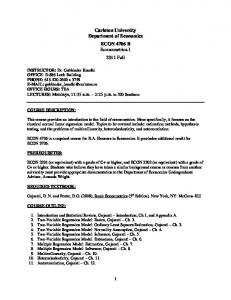
turbances in the workload or the system, and to maintain Service Level Agreements (SLAs). Disturbances in the workload include changes in the load intensity or the types of services requested. Disturbances in the system include failures or load imbalances, or responses to security attacks. A second goal of control is to optimize the use of resources. Control is based on observations of the ongoing Quality of Service (QoS), and of other system measures reflecting system status and activity, interpreted with the help of a performance model. The model in turn needs to reflect the system structure and behavior and provide means to infer current and future changes in the system. Figure 1 shows an application offering a service interface to system users at the top right. System measures at the bottom drive an autonomic control loop, which tracks and updates a model, makes decisions based on the model, the SLA, and other system goals, and makes the controlled changes. Control strategies have been described based on different kinds of performance models, including regression functions, queuing models [14] [15], and dynamic models [1][3][6][7][13]. In [12], the present authors described a hierarchical structure of models and controllers, and suggested the use of layered queuing models to quantitatively assess the effect of component and application tuning or provisioning on the performance of the application. Layered queuing models [4][5][17] are extensions of Queuing Network models [8], which capture contention for software resources such as threads and critical sections, as

well as for hardware. This paper assumes the use of layered queues, which are described further in Section 2. QoS targets

User services (Web Application Interface)

Model

Control Decision change Application Disturbance change

Model-Building Monitoring (Tracking Filter) QoS achieved, and other system measures

Figure 1 Architecture of an autonomic control loop based on a tracking model An important aspect of the autonomic control loop in Figure 1 is the model-building element. Its role is to maintain accurate model parameters as the system evolves. In tracking changes in the model parameters, various kinds of data give useful but indirect information. Some means is needed to integrate this data, in order to estimate the model parameters. In [20], it was proposed to integrate performance data and track the parameters of queuing models with a tracking filter. A tracking filter updates past estimates of parameters from observations on functions of them (such as performance observations), based on a performance model and a statistical model of the dynamic parameter change. Tracking filters are used in many fields, but not yet in computer system control. This paper evaluates the effectiveness of the filter mechanism for tracking parameters of a model of a time-varying layered system. The first application of a tracking filter to performance model parameter estimation in [20] used an Extended Kalman Filter to estimate the parameters of a queuing network with unknown but constant parameter values. The transient response of the filter when it first acquired the parameter value was evaluated under a wide range of conditions. The filter showed: • Almost instantaneous convergence to the transient parameter change

•

Low sensitivity to tuning parameters that describe the measurement accuracy and the parameter drift process This work extends [20] to evaluate the success of the filtering approach to track a timevarying parameter in a layered queuing model. The novel aspects of this work are: •

Evaluation of the effectiveness of approximations needed to make the filter practical

•

The use in the filter of an approximate sensitivity matrix for the layered queuing network

•

The interaction of the rate of system change, the system measurement accuracy, and the length of the measurement steps, in determining the accuracy of tracking

A Kalman Filter is a model-based estimator for time-varying state values in a dynamic system that can be derived either as an optimal leastsquares estimator, or a Bayesian estimator. At each step, the filter compares measured values (in our case, performance measures) to predicted values from a model, to give a prediction error e. From e, it updates the state estimates x with a linear update equation: xnew=xold+Ke. The Kalman gain matrix K is a function of certain properties of the model and of estimates of the accuracy of both the measurements and the model, which are also updated by the filter. K is updated at each step to minimize the mean of the square of the prediction error e (or the mean of a quadratic norm on a vector e). Details are given in Section 2. Kalman Filters were originally derived for estimating states of a linear dynamic system [10], and were extended to provide an approximately optimal filter for parameter estimation and for estimating states in non-linear systems. The Extended Kalman Filter is heavily used to estimate positions in space from radar data (see [2]). There is a vast literature on Kalman Filters; the references cited provide further background. The remainder of the paper is organized as follows. Section 2 describes a Web application and its layered queuing performance model; Section 3 explains the Extended Kalman Filter and its implementation for tracking layered queuing parameters; Section 4 presents the experiments and the results. The practical implementation issues of

the Kalman Filter are detailed in Section 5, and conclusions are presented in Section 6.

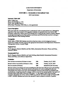
2. Time-varying Web Application We consider a Web-based application and its associated layered queuing model structure as shown in Figure 2. In terms of Figure 1, the Web application represents the controlled Application while the layered queuing model is the Model element in the autonomic control loop. In this section, we identify the structure of the performance model, the directly measurable data, the indirectly measurable data and the change characteristics of the above. requestPage [thinkTime=Z s.]

User (N users) (host)

(1) retrievePage [Sw ms]

Net (delay)

dbOp [Sd ms]

Database

(host) NetP (physical)

(host)

(0.2)

(0.4)

(1) netdelay [50 ms]

Workstations

WebServer (M threads)

DBProc

diskOp [15 ms]

Disk

WSProc

(host) DiskDev

Figure 2. The Layered Queuing Model of a Web application, showing its organization The User block in Figure 2 represents N separate users and their browsers, which alternately send requests to the Web Server every Z ms. (as a default, Z = 1000). Z is known as the think time. The WebServer block represents the server software with M threads, running on processor WSProc (indicated by the “host” relationship). The model represents M servers with a single queue of user requests. The box labeled RetrievePage represents the operation done for the users, and requires a CPU demand of Sw ms (default value 5 ms), one network latency of 50 ms, and on average 0.4 database operations and 0.2 disk operations. The disk and the database are here represented as single servers with a queue, running on their own devices DBProc and DiskDev, with CPU demands of Sd (default value 10 ms) and 15 ms, respectively. We will consider this model as a representation of a Web-based application system with a similar structure and the same structure of re-

quests between its components. In a real system, the behaviour of the components would be more complex than in the model, and the structure could contain more detailed substructures. For instance, a real database server would include threads, concurrency control mechanisms, and perhaps its own storage subsystem. For this study, we will represent the real system by a simulated system with the same structure as Figure 2. In this way, we can study the success of the tracking filter in tracking the parameters of the simulated system, if they vary.

2.1 Parameter Changes Figure 2 shows five parameters as variables: N = number of active users (default 100) M = number of Web-server threads (default 50) Z = mean User think time per request (default 1000 ms) Sw = mean Web server demand per user request (default 5 ms) Sd = mean database server CPU demand per database request (default 10 ms) A major challenge to autonomic systems is variation in offered load arriving at a service center. This phenomenon can be modeled by variations in Z or in N; a larger N or a smaller Z leads to a higher level of offered load. Variation in the type of transaction being executed by users is a second challenge, and it can be captured by variation in the CPU demand, or the request frequencies. CPU demands in a data centre can also vary because of provisioning (upgrading or downgrading the hardware). We will vary Z and the CPU demands, and keep N and the request frequencies constant. We assume that the system has parameters that change over time, according to a parameter change process as follows: •

Changes in some parameter a occur at discrete random instants, at a mean rate of αa changes/s, and the parameter values are constant between changes

•

At a change point, the new value a’ is independent of the previous value a, and is governed by a distribution with density function f(a), mean ma , variance σ2a, and coefficient of variation Ca = σa/ ma

The amplitude and frequency of this change process are characterized by Ta = 1/αa, the mean time between changes for a, and by Ca. There might be other change processes, such as a smooth process of gradual increments over time. For simplicity, we assume that only Z and Sd change. Thus, for tracking purposes, the parameter vector is a = [Z] or a = [Sd].

2.2 Performance Measures The directly measurable performance data would be taken, in a real system, from instrumentation and operating system counters. In our simulation, we consider: • Mean response time to users (R) • Utilization of the Web server processor(Uw) • Utilization of the database processor(Ub) • Utilization of the disk(Ud) Thus the measurement vector is z = [R, Uw, Ub, Ud], averaged over a measurement time interval of length T. Other measures might be of interest, such as quantiles of response time, or the probability of exceeding a stated target response time. However, the measures above are well understood and will give us a first view of the capability of tracking. Values for the think time Z, or the CPU demands Sw or Sd are not directly accessible at run time. They also vary over time, so we compute and track them indirectly by using the Extended Kalman Filter and the layered queuing models. The next section describes the tracking filter, which deduces these hidden measures from the measures that are available.

3. The Tracking Filter The filter takes the standard form of an Extended Kalman Filter (EKF) as described, for instance, in [2]. It applies to cases where there is a model xnew = f(x old) for the evolution of the desired state-and-parameter vector x, and a model z = h(x) for the relationship between the observation vector z and x. Here, we replace x by our unknown parameter vector a. In Kalman’s classic paper [8] the relationships f and h were linear and an optimal (least-squares) estimator was derived; in the extended filter the relationships are non-

linear and the optimality is only approximate. In our case, f is the identity, but h is a nonlinear function. In the discrete time filter used here, time advances in steps of duration T, indexed by a step counter k. The change process of the parameter vector ak is modeled as a drift driven by random increments: ak = ak-1 + wk-1 (1) The random vector wk has a mean of zero and has the disturbance covariance matrix Qk (which we assume to be a constant Q), and is independent from one step to the next. The system observation vector zk is modeled as a function h(ak), defined in our case by the relationship that determines the performance from the parameters, including an error of measurement. Thus, it assumes: zk = h(ak)+ vk (2) The assumed random error vector vk has a mean of zero, is independent from one step to the next, and has the measurement error covariance matrix Rk. The filter assumes that the relationship h is given by a performance model, the layered queuing model for the system, which includes the parameter vector a.

3.1 The Filter Computations The filter computations are recursive, beginning from an initial estimate a0, and an initial error covariance matrix P0. Each recursive step can be summarized as follows: (1) Based on the most recent parameter estimate ak-1, the filter predicts the measurements as h(ak-1) (because the assumed drift has zero mean, the predicted parameter value is the same as the previous estimate). From the current observation vector zk, it computes a prediction error vector ek: ek = zk - h(ak-1) (3) (2) The core filter calculation is the update of the estimates by the linear feedback equation: (4) ak = ak-1 + Kk ek where the “Kalman Gain” matrix Kk is computed as follows:

(a) Computation begins from an estimate Pk of the covariance matrix of estimation errors for ak . Pk is projected forwards one step, based on the drift covariance matrix Q: P-k = Pk-1+Q (5) (b) Then the optimal gain matrix Kk (which is only suboptimal when h is a nonlinear function, as it is here) is given by: Kk =P-kHkT(HkP-kHkT + Rk)-1 (6) In this equation, the matrix Hk is the matrix of partial derivatives of the performance model function h, with respect to the parameters a at their current values ak-1. Thus, Hk is a matrix of sensitivity values for the performance model. (3) When ak is updated, the covariance estimate Pk is also updated, to take into account the improved accuracy after the filter step: Pk=(I-KkHk)P-k (7) Where there is no ambiguity, the step subscript k will be omitted. Figure 3 shows the organization of the filter. Model h (x) a: new parameters

System (Web app)

z=h(x): predicted H: sensitivities performance

Kalman Filter a, P: new parameters and covariances

e: prediction error

Monitor z: measured performance

Figure 3. The Kalman Filter architecture The optimality and convergence properties of the EKF depend on the way the functions are linearized around the current estimate of a [11]. This Extended Kalman Filter (EKF) [2][19] linearizes f(a) and h(a) by a first order Taylor series around the state estimate â-k-1 and does not take linearization errors into account. A variant called the Iterative Kalman Filter (IEKF) linearizes h(a) around the predicted state estimate ak-1. Other variants of the filter, like the Unscented Kalman Filter [9] or the Divided Difference Filter [16] capture the linearization errors in the covariance matrices. They were shown in [11] to provide better estimates when dealing with non-linear f(a)

functions, while EKF and IEKF provide better performance when dealing with non-linear h(a).

3.2 The Influence of the Filter Parameters The matrices Q and R capture knowledge or assumptions about the disturbances and the measurement errors, and they also influence how the filter reacts to new data. Both Q and R can often be assumed to be diagonal, with variance terms for the one step disturbances and the measurement errors, respectively. Small values in Q indicate that only small changes are expected, and lead to a small filter gain matrix K that can only adapt slowly. A large value of Q leads to large P and thus large gains that might overreact to measurement errors. Each diagonal element Qii should be set to the square of an estimate of the magnitude of the changes to be tracked in parameter ai: Qii = (approx. magnitude of change in ai)2 Each diagonal element Rii should be an estimate of the variance of the measurement error in zi. If the averaging time T is large enough (which we shall assume is the case) Rii varies as: (8) Rii = const/T A standard step-length T* was determined (by experiment) that gave a 95% confidence interval of +- 5% in the user response time measure z1. For the system in Figure 2 with the default values of the parameters, T* = 15.7s. From the asymptotic properties of the t distribution, the confidence interval is 1.96 times the standard deviation. This implies that when T = T*, R11 = (0.05 (mean of z1)/1.96)2. For other values of T, the ratio of T to T* is denoted by γT: γT = T / T* and then, approximately: R11 = (0.025 (mean of z1))2/ γT This value could be used in the filter, with the model prediction to estimate the mean of z1. Further, it can be assumed that the confidence intervals of the other measures have similar accuracy. Thus: Rii = (0.025 (mean of zi))2 / γT

(9)

To demonstrate the ability of the filter to follow parameter changes, the system in Figure 2 was simulated with deterministic and random parameter changes (disturbance changes). A tracking filter was set up, based on the same model solved by an approximate analytic calculation with the LQNS solver. The filter was driven by the measurement vector defined above, made up of the user response time and the device utilizations: z = [R, Uw, Ub, Ud] These are typical of readily available performance measures from a real system. Changes in a single parameter were tracked, with either Z or Sd. The goodness of tracking can be measured in two ways, by the performance prediction error ER or by the parameter tracking error EA. We will use the RMS (root-mean-square) tracking error measures for both of these quantities.

4.1 Tracking Deterministic Changes in Parameters The tracking performance was recorded for a series of alternating step changes in value of two parameters: •

User think time Z (which affects the arrival rate; smaller Z gives a higher arrival rate)

•

Database service time Sd

Case 1: Z alternates between 500 ms and 2500 ms with a change every 471 s. (30T*). This creates a much larger arrival rate for small Z than for large Z (about 168/s when Z = 500, vs 39/s when Z = 2500). Equivalently, we could have modified the arrival rate directly. The filter parameters were set to: •

T = T* = 15.7 s. (making γT = 1). This gives an estimation accuracy such that the 95% confidence interval in the mean user response time is +-5% at the base case parameters.

•

Q = 4,000,000. Q is a scalar, since there is just one parameter to track, and this is the square of the step change in Z that is applied in going from 500 to 2500.

•

Rk was a diagonal matrix with an element for each performance measure. From Eq. (9), the ith element is Rk,ii = (0.025*hi(ak))2

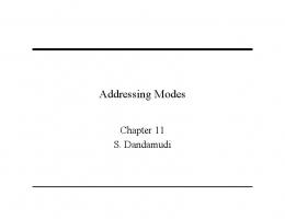
Figure 4 shows a fragment of the record of values taken from the simulation and the tracking filter. The filter tracks the change in Z with a onestep delay plus a few steps to settle to the new value.

3500 3000 Think Time

4. Results

2500 2000 1500 1000 500 0 1

16

31 46 61 76 91 106 121 136 151 166 Time Sequence

real value tracking value

Figure 4 (Case 1) Tracking performance for a deterministic sequence of mean user think times. (T = T*) The high and low values of Z give a moderate load and a heavy load on the system, respectively. Thus the performance calculations traverse the knee in the performance curves between these two regimes, where the function h is the most nonlinear. The tracking error is visibly greater for Z = 2500. The arrival rate is lower, and there are fewer response times in the averaging period, so the variance of the measurement error is larger than is allowed for by R when it is calculated by Eq. (9). The variation of measurement errors with load is quite a complex phenomenon, and Eq. (9) makes the simplifying assumption that the relative accuracy is constant in a neighborhood of the configuration for which it was measured (in establishing T*). This assumption allows constant values to be used for Q and R. The assumption is justifiable if the sensitivity to R is low. Figure 4 supports the assumption, in that the tracking errors at both extremes are moderate. Further tuning of Q and R might give even better performance.

60

3000 2500 2000 1500 1000 500 0 1

10

19

28

37

46

55

64

Time Sequence

73

82

91 100

Real Value Tracking Value

Figure 6. A trace fragment of tracking random changes. Experiments were done for a range of values of the measurement step time T, the rate of changes α, and the variance of the changes σ2. The time T*, which is characteristic of the system and designates the time to get a moderately accurate average by measurement, was used to normalize these values. The normalized relative parameter change rate, γα, specifies the change rate relative to T*: γα = αT*. As already defined, the normalized relative measurement interval γT specifies the measurement interval T relative to the time T*:

50 DB Demand

Figure 6 shows a fragment of a trace of the filter tracking random changes in the mean User think time. Sometimes the “real” mean value used by the simulation (the line with the diamonds) changes in the middle of a measurement step, so there is a point between two values. Generally, the filter follows a change within a few steps.

ThinkTime

Case 2: The database demand Sd alternates between 10 ms and 40 ms, with changes every 471 s. At the lower value, the system is lightly loaded; the higher value creates a significant load at the database, with a queuing delay that blocks some application threads. Q was set to 900, and R was set as in Case 1. Figure 5 shows how the filter tracked the changes, corresponding to Figure 4 for Case 1. Again, the filter takes a few steps to track the (very large) change. In this case, the larger tracking errors are evident for the larger value of Sd, which corresponds to a heavier load (as opposed to the case above in which the larger value of Z gives the lighter load). This time the number of responses in an averaging period decreases with heavy load, since the delays at the server back up the traffic. Also, there is a general tendency for the accuracy of statistics to suffer as system load increases, because of increased correlation of the successive responses. This dependency is complex and was not accounted for in setting R according to Eq. (9). Again the system is traversing through the most nonlinear range of the performance relationships expressed in h(a).

40 30 20 10 0 1

15 29 43 57 71 85 99 113 127 141 155 169 Time Sequence

real value tracking value

Figure 5. (Case 2) Tracking of deterministic changes in the database service time Sd .(T= T*)

4.2 Tracking Random Changes in Parameters A random change process was generated in the simulation, with step changes of a parameter value occurring at randomly chosen instants (multiples of a common time step), at a mean rate of α changes/s. The change process was applied to one parameter at a time, first to Z and then to Sd.

γT = T/T* Base values of these parameters in the following experiments were γα = 0.025 and γT = 4. At each change instant, a new value of the parameter (Z or Sd) was chosen independently according to a shifted hyper-exponential distribution (such as: Z = constant + random part), which had a mean value equal to the average value of the parameter and a stated coefficient of variation C. The base value of C was C = 1, but in Case 7, C was varied from 0.1 to 2. Case 3: Parameter Tuning. The filter tuning parameters Q and R might affect the way the filter reacts. Small entries in Q

make the filter conservative, as it assumes only small changes are possible in a single step. Small entries in R make the filter track more aggressively, as it assumes that the measurements are accurate and therefore the filter must react in order to explain them. We must learn how to set these parameters, and also it is important to understand how sensitive the whole filter process is to their values. To investigate these effects, the entries of Q and R were multiplied by factors denoted as QFac and RFac respectively. These two factors were varied over two orders of magnitude. Otherwise, the experiments had the usual base values of γα = 0.025, γT = 4.0 and CVa= 1.0. The expressions used for Q and R were: Qii = (QFac(mean of ai)CVai)2 (9a) Rii = ((RFac) (zi) / 1.96)2 /γT

(9b)

Table 1. (Case 3) The RMS tracking error in the mean user think time Z, as R and Q are varied RFac

QFac 0.01

0.025

0.05

0.1

0.25

0.5

143.7

143.7

131.2 143.7

1

2

0.02

124.6

140.0 143.7

143.8

144.6 2.72E7

0.05

156.4

124.6

143.8

143.8

143.8

143.6

0.1

186.4 145.9 124. 6 131.2 143.8

143.8

143.8

143.8

0.2

221.1

176.1 145.9

140.0 143.8

143.8

143.8

0. 5

264.8

221.1

186.4 156.4

131.1 143.7

143.8

1

290.6

255.1

221.1

186.4 145.9

2

317.0

282.6

255.1

221.8

176.1 145.9

124.6

131.0

4

345.1

308.1

282.6

255.1

290.9 176.1 145.9

124.6

124.6

124.6

124.6

131.2 143.7

The results in Table 1 show that it is the ratio of Q to R that is important, rather than the values of the parameters. Also, above the diagonal (when Q is too large, and the filter over-responds to measurement errors), there is only a modest effect up to the point in the top right corner, where the error explodes. On the other hand, when Q is too small (the filter is sluggish), the error increases steadily. We can conclude that the tracking performance is somewhat insensitive to Q and R. Around the ideal balance between Q and R, there is a wide band (more than a factor of 10 up or down) in which the filter is “not bad” (within a factor of 2 in RMS tracking performance). This agrees with the results reported in [20] for transient response

and queuing models. Furthermore, it is better if Q should be somewhat overestimated (rather than underestimated) relative to R. For the rest of the paper, we set QFac =0.1 and RFac = 0.2. Case 4: Measurement Time The next investigation considers how the measurement step time affects the accuracy of tracking. The mean number of parameter changes per measurement step is given by the ratio αT, for a given parameter change process with mean rate of α changes/s. We expect that low values of this ratio, such as αT