arXiv:cond-mat/0001429v1 29 Jan 2000. Tractable non-local ...... (A16). This is our most general result, which reduces to Eq. (19) when Ç«k(0) = Ç«k(L). Note that in the .... 30 D. Pines, Elementary Excitations in Solids (W. A. Ben- jamin, Inc, New ...
Tractable non-local correlation density functionals for flat surfaces and slabs Henrik Rydberg and Bengt I. Lundqvist Department of Applied Physics, Chalmers University of Technology and G¨ oteborg University, S-412 96 G¨ oteborg, Sweden
David C. Langreth and Maxime Dion
arXiv:cond-mat/0001429v1 29 Jan 2000
Center for Materials Theory, Department of Physics and Astronomy, Rutgers University, Piscataway, New Jersey 08854-8019
gained from choosing a particular sub-class of response functions, utilizing a differential formulation and sparse matrices, and recognizing the insensitivity to the details of the density profiles, simplifications which might transfer even to three dimensions. The ubiquitous van der Waals force plays an important role for numerous physical, chemical, and biological systems, such as physisorption,16,17 vdW complexes,18 vdW bonds in crystals, liquids, adhesion, and soft condensed matter (e.g., biomacromolecules, biosurfaces, polymers, and membranes).18,19 The DFT expresses the ground-state energy of an interacting system in an external potential v(r) as a functional E[n] of the particle density n(r), which has its minimum at the true ground-state density.1 The Kohn-Sham form of the functional makes the scheme a tractable one, as it leads to equations of one-electron type, and accounts for the intricate interactions among the electrons with an exchange-correlation (XC) functional Exc [n].2 This XCenergy functional can be expressed exactly as an integral over a coupling constant (λ),20,3,21 the so-called adiabatic connection formula (ACF),
A systematic approach for the construction of a density functional for van der Waals interactions that also accounts for saturation effects is described, i.e. one that is applicable at short distances. A very efficient method to calculate the resulting expressions in the case of flat surfaces, a method leading to an order reduction in computational complexity, is presented. Results for the interaction of two parallel jellium slabs are shown to agree with those of a recent RPA calculation (J.F. Dobson and J. Wang, Phys. Rev. Lett. 82, 2123 1999). The method is easy to use; its input consists of the electron density of the system, and we show that it can be successfully approximated by the electron densities of the interacting fragments. Results for the surface correlation energy of jellium compare very well with those of other studies. The correlation-interaction energy between two parallel jellia is calculated for all separations d, and substantial saturation effects are predicted. PACS numbers: 31.15.Ew,71.15.Mb,34.50.Dy,02.70.-c
I. INTRODUCTION
The density-functional theory (DFT),1 with its localdensity (LDA)2,3 and semilocal generalized-gradient approximations (GGA),4–7 is not only successful in numerous applications to individual molecules and dense solids. It is also under intense development, for instance, in order to include non-local effects, such as van der Waals (vdW) forces.8–15 The latter are needed in order to allow DFT to describe sparse matter. A unified treatment of vdW forces at large and asymptotic molecular separations is available,15 and a description at short distances and at overlap is striven for. An accurate calculation for the interaction of two He atoms has been given,12 and recently the first microscopic (RPA) calculation of the vdW interaction between two self-consistent jellium slabs has been reported and given a density functional (DF) account.14 The ultimate challenge is to construct an approximate vdW DF that is generally applicable, efficient, and accurate. We here propose an explicit form for the vdW DF that applies to flat surfaces, test it successfully against these slab results, and apply it to two parallel flat semi-infinite metal surfaces. This is a case with relevance for many physical situations, including wetting and atomic-force microscopy (AFM). Compared to the vdW-DF approximation proposed by Dobson and Wang,14 the virtues of our functional are the computational simplifications
Exc = −
Z
0
1
dλ
Z
0
∞
du Tr [χ(λ, iu)V ] − Eself , 2π
(1)
where V (r, r′ ) = 1/ |r − r′ | and where the density-density correlation function is denoted by χ(r, r′ , iu; λ).22 Eself is the Coulomb self-energy of all electrons, which is exactly cancelled by a corresponding term in χ(λ, iu)V . Equation (1) shows a truly non-local XC interaction and is a starting point for approximate treatments, local (LDA), semilocal (GGA) and non-local ones. The LDA and GGA are completely unable to express the vdW interaction in a physically sound way. The exact XC energy functional, on the other hand, of course encompasses such interactions.8 The basic problem of making DFT a working application tool also for sparse matter is to express the truly non-local vdW interactions between the electrons in the form of a simple, physical, and tractable DF. Equation (1) is then the starting point. Along these lines, we have proposed extensions of the DFT to include van der Waals interactions,8,9,11,13,15 with very promising results for the interaction between two atoms or molecules, an atom and a surface, and two parallel surfaces, respectively. This now unified approach15 applies for separated systems, i.e. when the electrons of the interacting fragments have negligible overlaps. 1
The corresponding asymptotic expressions have singular behaviors at short separations d. Yet one knows that the vdW forces are finite.23 They should go smoothly over to the XC forces that apply in the interior of each electron system. This phenomenon is often called damping, or saturation.24–26 Approximate saturation functions have been proposed, in particular for the cases of vdW molecules24 and physisorbed particles.25,26 The key difficulty in extracting the vdW DF from Eq. (1) is the computational complexity. A direct solution gives simply too many operations on the computer. The guideline for our reduction of the number of such operations is to exploit analytical advantages of RPA-like approximations, to focus on the key quantity, to recast the integral formulation into a differential one, leading to a sparse-matrix computation, and to make maximal use of symmetry. Our exploratory study here concerns cases with vdW forces between two flat parallel model systems. We first test our approximate functional on the model system of two self-consistent jellium slabs, utilizing the recent RPA results,14 which gives the size of the correlationinteraction energy per unit area, showing saturation. We then test our DF against accurate calculations of the surface correlation energy,27,28 showing an excellent agreement. After these successful tests we make predictions on two parallel semi-infinite jellia.
To simplify this expression and to get a functional in terms of the electron density n(r), we have to focus on the key target, the non-local part, introduce key quantities, and rewrite the expressions, in order to make physically sound and computationally efficient approximations. It is more convenient to introduce the polarizability or dielectric function instead of χ. ˜ The polarizability α (a matrix in the spatial positions) is defined by the relation P = α · E, where P is the polarization. We have δn = −∇ · P = −∇ · α · E = ∇ · α · ∇Φ,
so that from the definition of χ, ˜ one has χ ˜ = ∇ · α · ∇. In turn the dielectric function is given by ǫ ≡ 1 + 4πα. In terms of ǫ Eq. (3) then transforms to Z ∞ du Exc = Re [Tr [log(∇ · ǫ · ∇G)]] − Eself , (5) 0 2π where we have introduced the Coulomb Green’s function G = −V /4π and used ∇2 G = 1. The Tr [log] expression gives great advantage for the further analytical and numerical treatment. The only approximation made so far is the neglect of the coupling constant dependence of χ ˜ when doing the coupling constant integration. This is not an additional approximation either in the RPA or for the approximate ǫ’s we use here. In order to develop long-range functionals, one may substitute approximations for the dielectric function based on the free electron gas into Eq. (5). To obtain tractable expressions it will normally be necessary to make still further approximations. In this case it is desirable to use the additional approximations only for the non-local part of Exc so as to avoid destroying the accuracy of the LDA in the high-density regions. Ideally one would subtract from Eq. (5) the LDA version of the same approximation, and would envisage adding back a better version of the LDA. Here we make a similar, but more tractable subtraction, which takes the form Z ∞ du 0 Exc = Re [Tr [log(ǫ)]] − Eself . (6) 2π 0
II. GENERAL THEORY
The λ integration of Eq. (1) can be performed analytically in some cases, such as in the random-phase approximation (RPA). In 1957 Gell-Mann and Bruckner (GMB)29 presented the RPA correlation energy as a selected summation of ring diagrams, which gives a logarithmic form.30 Their study concerns the homogeneous electron gas, where equations simplify thanks to the three-dimensional translational invariance and plane waves. Here we treat systems with less symmetry. By virtue of the fluctuation-dissipation theorem, the density-density correlation function χ is equal to the density change δn induced by an external potential Φext , i.e. δn = χΦext . It satisfies χ(λ, iu) = χ(iu) ˜ + λχ(iu)V ˜ χ(λ, iu),
(4)
0 Exc has the property that it is a good approximation for a slowly varying system, becoming exact for a uniform system. For density variations slow on the scale of the range or width of ǫ(r, r′ ), it agrees with the LDA, the trace in Eq. (6) replacing the integral over density. Subtracting Eq. (6) from Eq. (5), one obtains Z ∞ � � �� du nl Exc = Re Tr log(ǫ−1 ∇ · ǫ · ∇G) . (7) 2π 0
(2)
where χ ˜ is the density response to a fully screened potential Φ, i.e. δn = χΦ. ˜ We assume here that the coupling dependence of χ ˜ can be neglected, when performing the λ integral in Eq. (1). This is true in the random-phase approximation, where χ ˜ is the density response function for λ = 0, and is also true for the approximate dielectric functions, which we use here. Equation (1) then becomes Z ∞ du Exc = Re [Tr [log(1 − χ(iu)V ˜ )]] − Eself , (3) 0 2π
We will call this the non-local exchange-correlation energy, although for models more general than those used in this paper, an additional short-range correction must 0 be applied to make Exc correspond precisely to the LDA, nl and hence to make Exc the deviation from the LDA. The approximations considered in this paper contain no non-local exchange component, in effect making
where the real part means the principal branch. 2
Eq. (7) our approximation for the non-local correlation energy Ecnl . Using this fact, together with Tr [log x] = log(det x) and ∇2 G = 1, we obtain Z ∞ du log det(1 + ǫ−1 [∇, ǫ] · ∇G) (8) Ecnl = 0 2π
Gk (z − z ′ ) = −
(13)
Since the logarithm of Eq. (7) can be expanded in powers, the integration over k may be singled out, and we may express the non-local correlation energy per surface area (A) as Z Z ∞ d2 k du nl log |det(1 + lk′ ∂z Gk )| . (14) Ec /A = (2π)2 0 2π
where the notation [A, B] means the commutator. We will later use the fact that Eq. (8) involves only the determinant to good advantage.
In Eq. (14), the determinant is given in terms of integral operators. To take advantage of the locality of the Laplacian, we use (∂z2 − k 2 )Gk = 1 to express it in terms of differential operators
III. METHOD FOR PLANAR GEOMETRIES
Now we are in a situation to discuss what ǫ to use. We will in this paper concentrate on the simple case of jellium systems. Our aim is to find an efficient way of exploring the planar translational invariance of the jellium system – not only to decrease the number of spatial integrations. The major difficulty in evaluating Eq. (8) is the determinant, which is O(N 3 ) in the general case, N being the number of grid points in a discrete representation. This holds true even in one dimension. So, instead of allowing a completely general ǫ, we aim at approximations resulting in differential operators only, for which the determinant is known to be O(N ), hence significantly simpler to calculate. In the particular case of planar translational invariance, i.e. for planar surfaces or slabs, we use an approximate form that is made local in the coordinate perpendicular to the surface, Z ′ d2 k ǫ(r, r′ ) = δ(z − z ′ ) ǫk (z)eik·(r−r ) , (9) 2 (2π)
φ , φ0
(15)
φ = det(∂z2 − k 2 + lk′ ∂z )
(16)
det (1 + lk′ ∂z Gk ) = where
and where φ0 is the empty space (ǫ = 1) value of Eq. (16). The step from Eq. (14) to Eq. (15) requires that the differential operators are defined throughout the whole space. Our ultra-fast method is made possible by the observation that the determinants in Eq. (15) can be written down, not only for the full system, but also for a subdivision of it. Related determinants for the subsystem satisfy a simple second-order differential equation as a function of subsystem size. Thus by a simple renormalization, one may evaluate Ecnl with the same effort as finding the charge induced by an applied electric field. A similar relation holds also in several dimensions, which will be explored in another paper. To make this more concrete, let us suppose that ǫk (z) varies only in the interval 0 < z < L (which will eventually be extended to infinity) and takes the same value at either end point. This is the case for parallel surfaces or slabs of identical materials. Then for each value of z we can define a determinant φ(z) for the subsystem extending from 0 to z. It is clear then from Eqs. (14), (15), and (16) that Ecnl is given by Z ∞ Z du d2 k φ(L) nl Ec /A = lim log . (17) L→∞ 0 2π (2π)2 φ0 (L)
where k is a wave vector parallel to the surface. Keeping the fully non-local form along the symmetry plane allows, e.g., the effect of the cutoff, which was introduced artificially in previous approximations of this type,31,15 to occur in a natural way laterally. The first thing we note about Eq. (9) is that we easily form the inverse Z ′ d2 k −1 ′ ′ ǫ (r, r ) = δ(z − z ) ǫk (z)−1 eik·(r−r ) . (10) (2π)2 Evaluating the commutator then yields Z d2 k ǫ′k (z) ik·(r−r′ ) ǫ−1 [∇, ǫ] = zˆδ(z − z ′ ) e , (2π)2 ǫk (z)
1 −k|z−z′ | e . 2k
(11)
As discussed in Appendix A, the determinants φ(z) and φ0 (z) individually have oscillating signs that do not occur in their quotient. However, the envelope determinants ˜ φ(z) and φ˜0 (z) can be scaled so that they satisfy the simple differential equation
where the prime indicates differentiation with respect to z. In what follows we shall substitute l(z) = log(ǫ(z)), yielding l′ (z) = ǫ′ (z)/ǫ(z). In the same basis we express the Green’s function, Z ′ d2 k ′ Gk (z − z ′ )eik·(r−r ) , (12) G(r − r ) = (2π)2
˜ (ǫk φ˜′ )′ = k 2 ǫk φ,
(18)
˜ together with the boundary conditions that φ(0) = 0 and ˜ ˜ we obtain φ(L) = 1. In terms of φ,
where 3
Ecnl /A
= − lim
L→∞
Z
0
∞
du 2π
Z
φ˜′ (0) d2 k log ′ , 2 (2π) φ˜0 (0)
the plasma frequency ωp as q → 0, and then a dispersion with a limiting behavior ωq → q 2 /2m, the kinetic energy of one electron, in the impulse-approximation, valid in the Compton-scattering limit, q → ∞. In the electron-plasmon coupling one focuses on the magnitude and position of the sharp plasmon peak, and neglects the broadening, i.e. ǫ is described in a plasmon-pole approximation.33 A dispersion law like
(19)
where the prime indicates differentiation with respect to z, which in this case is the subsystem size. However, note that φ˜ is also just the electrostatic potential as a function of distance z, within a system having a potential difference across it along with a prescribed variation in ǫ. Thus the calculation of the determinant becomes a simple electrostatic problem which is easily solved. To illustrate this, consider the case of two identical parallel surfaces a distance d apart, when d is much larger than the thicknesses of the surface-healing layers. Solving Eq. (18) for the described boundary conditions then becomes a trivial matching problem (see Appendix B), which after insertion into Eq. (19) immediately leads to the Lifshitz formula32,13 Z ∞ Z du d2 k Ecnl /A = log 1 − ρ2 e−2kd + 2γnl . (20) 2 (2π) 0 2π
ωq2 = ωp2 + (vF q)2 /3 + (q 2 /2m)2
has been shown to efficiently account for the average behavior of plasmon-like excitations and for correlation properties of the homogeneous electron gas.33 Introducing the electron density via ωp2 (z) = 4πn(z) and vF (z) = (3π 2 n(z))1/3 in Hartree units, n(z) being the electron density profile in this planar case, the dielectric function can be written as ǫ(z, k, iu) = 1 +
ωp2 (z) , (23) u2 + (vF (z)q(k))2 /3 + q 4 (k)/4
where the imaginary frequency ω = iu is introduced. Alternatively, Eq. (23) may be viewed as an interpolation between the exact small- and large-q behavior of the Lindhard expression for the frequency-dependent dielectric function. However, we see little point in using such an elaborate expression, since our concern here is to investigate how well local approximations to the dielectric function work in highly non-uniform systems. In directions parallel to the surface, our approximation Eq. (23) allows fully for the non-diagonality of ǫ with respect to the corresponding spatial coordinates, as implied by a Fourier transform with respect to the parallel wave vector k. However, in directions perpendicular to the surface, our approximation takes ǫ to be diagonal in the coordinates z and z ′ . It is thus taken to be local not only in this sense, but in the additional sense that it is a function only of the local density. To compensate, we retain the corresponding component q⊥ of the wave vector q in the right side of Eq. (23) as a parameter, so 2 . We thus take 1/q⊥ to be that everywhere q 2 = k 2 + q⊥ a constant measure of length over which ǫ is effectively nonlocal. The dispersion perpendicular to the surface in Eq. (22) is in this way replaced by a parameter that we will fix to some length scale appropriate for the surface. For physical reasons such a length scale should be associated with intrinsic electron-gas parameters like the screening length or the extent of the correlation hole. There are of course several choices available. It must be kept in mind that we are after long range surface properties in a variety of environments. These properties are determined by various response functions introduced by Feibelman,34 of which the simplest, R dz znind (iu, z) d(iu) = R , (24) dz nind (iu, z)
Here ρ = (ǫb − 1)/(ǫb + 1), ǫb being the bulk dielectric function, and γnl is defined by γnl = (Ecnl (d → ∞) − Ecnl (0))/2A.
(22)
(21)
Since, by construction, Ecnl = 0 for a uniform (d = 0) system, γnl may equivalently be defined as the non-local correlation contribution to the surface tension of a single surface. The original ACF Eq. (1) is now reduced to a set of simple electrostatic calculations, each one being an O(N ) operation instead of O(N 2 ), a major simplification. Of course the success of the method depends on how well we can reproduce the true dielectric function using our approximate form Eq. (9). The only approximation made so far is the assumption of a local dielectric function perpendicular to the surface. IV. APPROXIMATE DIELECTRIC FUNCTION
Equation (17) or (19) provides the basis for a functional that describes the van der Waals interaction between planar objects. To turn these equations into density functionals, we have to introduce quantities that depend on the density n(r). Our suggestion is based on an approximate dielectric function ǫk that depends on the local density n(r). It utilizes experiences from the homogeneous electron gas and from experimental h studies of i 1 the dynamical structure factor S(q, ω) ∝ Im ǫ(q,ω) −1 , where ¯hq and h ¯ ω are the momentum and energy losses, respectively, of a photon or a charged particle being scattered while passing a bulk sample. There is a peak in S(q, ω), the plasmon peak, sharp in the ideal electron gas and of varying width in real materials. This peak carries most of the spectral strength and has ω equal to
is the centroid of induced charge when a uniform electric field is applied perpendicularly to the surface. However,
4
q⊥ > 0 affects the k → 0 limit of Eq. (23). This also means according to Eqs. (26) and (27) that the van der Waals planes will be predicted to be somewhat too far from the surfaces in this approximation. The d-function, i.e. Eq. (24) will also be too large, significantly so at small u. Far more important, though, is the fact that our simple dielectric function reproduces the dynamic properties of the D-function very well, as shown in Figures 1 and 2. Thus the overall scaling properties of our theory in a variety of non-uniform van der Waals environments should continue to be correct.
for the van der Waals properties of a planar surface, a related function D(iu) as defined by Hult et al.,11 D(iu) =
ǫb (iu) − 1 ǫb (iu) d(iu), ǫb (iu) + 1 ǫb (iu) + 1
(25)
is more important.35,36,25,37 In particular the D-function arises in connection with the calculation of van der Waals planes, which are determined not only by the D of the surface in question, but also by a response function of the other body. For example, for a surface in the vicinity of an isotropic atom, the van der Waals plane Z is given by35,25,37,11 Z ∞ 1 ZvdW = du α(iu)D(iu), (26) 4πC3 −∞
1.6 1.4
where α(iu) is the polarizability of the atom and C3 is the coefficient of the leading 1/z 3 term in the asymptotic form of the interaction energy. In order for the surface calculation to scale correctly for a wide variety of atoms with different α(iu)’s, it is obviously important for our approximation to well reproduce D(iu). Similarly, for two parallel surfaces labeled A and B, the van der Waals plane for surface A is given by Z ∞ 1 A = ZvdW du ρB (iu)DA (iu) + ∆Z A , (27) (4π)2 C2 −∞
D(iu) (a.u.)
1.2 1.0
Present calculation Hult et al. TDLDA
0.8 0.6 0.4 0.2
where ρB (iu) is the long wavelength surface response B function of surface B, ρB (iu) = (ǫB b (iu)− 1)/(ǫb (iu)+ 1), 2 and C2 is the coefficient of the leading 1/z term in the asymptotic form of the interaction energy. The main difference in cases such as this one, where two infinite bodies are involved, is that terms involving multiple reflections no longer vanish in the asymptotic limit, and should be explicitly included as indicated by the ∆Z A term in Eq. (27). However, it is common experience that in the asymptotic limit multiple reflection terms are typically small enough to treat in perturbation theory,38,13 a conclusion that we agree with. Therefore, the first term in Eq. (27) is dominant, and the conclusion that D(iu) is the key quantity to obtain accurately remains. Note, however, that in the numerical calculations presented later, the full form of Eq. (27), including all multiple reflections (see Eqs. (8) and (9) of Ref. 13), is used. Thus we opt to choose q⊥ based on the premise that the D-function should be reproduced accurately. We implement this by choosing q⊥ so that D(0) agrees exactly with full LDA calculations of this quantity, a procedure precisely analogous to that of Ref. 15. In this way, the parameter q⊥ may be indirectly determined as a function of the electron gas parameter rs . This determination gives q⊥ ∼ 1/rs ∼ kF as expected from previous arguments. The constant q⊥ smoothly limits the response at small k and small u values. It thus replaces the sharp cutoff used in the earlier scheme.15 In doing this, we consciously violate the Lifshitz limit, obtaining somewhat smaller vdW coefficients than Ref. 13, since the choice
0.0 0.0
0.2
0.4
0.6
0.8
1.0 u/ω p
1.2
1.4
1.6
1.8
2.0
FIG. 1. The D-function D(iu) for a jellium profile of rs = 2. Solid line: Present calculation. Dotted line: Reference 11. Circles: D-function based on a TDLDA calculation.39 1.4 1.2
D(iu) (a.u.)
1.0 Present calculation Hult et al. TDLDA
0.8 0.6 0.4 0.2 0.0 0.0
0.2
0.4
0.6
0.8
1.0 u/ω p
1.2
1.4
1.6
1.8
2.0
FIG. 2. The D-function D(iu) for a jellium profile of rs = 4. Solid line: Present calculation. Dotted line: Reference 11. Circles: D-function based on a TDLDA calculation.39
5
TABLE I. Static and dynamic image-plane positions (a.u.) of the jellium surface, calculated as a function of rs .
0.45
q⊥ (a.u.)
0.40 0.38 0.35 0.33
q⊥ from LDA data q⊥ = 0.416e−0.217rs + 0.168
0.30
D(0)a 1.57 1.55 1.48 1.41 1.35 1.32 1.24 1.17
rs 2.00 2.07 2.30 2.66 3.00 3.28 4.00 5.00
0.43
a
D(0)b 1.57
ZvdW c 1.15 1.15 1.15 1.14 1.13 1.14 1.12 1.09
1.35 1.25 1.17
ZvdW d 0.96
0.87 0.79
This work. b Reference 40. c This work. d Reference 13.
0.28 0.25 2.0
2.5
3.0
3.5 rs (a.u.)
4.0
4.5
Eq. (28) are compared to those of a recent RPA calculation of a slab system of rs = 2.07 by Dobson and Wang,14 as well as to those of their approximate DF (IGADEL). The saturation effects are found to be substantial in this small-separation region, and we judge all the proposed density functionals in the figure to give good accounts of the non-local correlation energy. The agreement with IGADEL reflects the inherent similarities between IGADEL and our approximation. The tractability of the latter is however not reflected in the table, but has to be stated here (about a thousand times faster than IGADEL for this particular system, due to the overall lower computational complexity of our DF), together with the claim that this gives great prospects for a tractable future general DF. The calculation presented in Fig. 4 is performed using a simple superposition of the densities of two separate slabs (obtained from d = 12 data) as input. The difference between the non-local correlation energy for the
5.0
FIG. 3. Optimal values of q⊥ , calculated for jellium surfaces of different densities, described by rs . Circles: Optimal q⊥ as a function of rs , calculated from LDA data.40 Solid line: Equation (28).
In order to investigate the approximation with regard to key properties, we use as input to our functional a set of self-consistent single-surface jellium densities in the metallic range (rs = 2−5). The exact form of the density profiles is however not that important; by construction, a non-local energy is expected to depend less sensitively on the exact form of the density, and results in this paper show that this is indeed the case. The optimal q⊥ values found by fitting to the values of D(0) of Ref. 40 are shown in Fig. 3 as a function of the electron-gas parameter rs , well accounted for by the simple interpolation formula q⊥ = 0.416e−0.217rs + 0.168.
0
(28)
The variation is roughly 50 percent over the whole metallic range, indicating a rather small overall sensitivity. Table I shows how the quantities D(0) and ZvdW varies with rs , using the parameterization Eq. (28). In the fourth and fifth columns, the values of the present method for the van der Waals plane ZvdW are compared to those of Ref. 13. Although the slightly larger coefficients are expected from considerations earlier in this section, the fact that the numbers come out almost independent of rs is somewhat of a surprise.
(Ecnl(d) − Ecnl (∞))/A (ergs/cm2)
−100
−200
−300
Present calculation Present calc., SC dens. RPA−LDA IGADEL−LDA
−400
−500
−600
V. RESULTS −700
To test our approximate DF, we solve Eq. (18), using Eq. (23), and insert the result into Eq. (19) for a known system, consisting of two parallel jellium slabs, separated by a distance d. Figure 4 shows results in ergs/cm2 (ergs/cm2 = 0.6423 µHa/a20 ) for the non-local correlation-interaction energy per surface area, (Ecnl (d) − Ecnl (∞))/A. The results using the rs = 2.07 value of
0
1
2
3
4
5
6
7
8
9
10
11
12
d (a.u.)
FIG. 4. Small-separation (d) variation of the non-local correlation-interaction energy (ergs/cm2 ) between two parallel jellium slabs of rs = 2.07 and width 5 a.u.14 Solid line: Present calculation. Stars: Same calculation but using the self-consistent densities of Ref. 14. Circles: RPA−LDA of Ref. 14. Diamonds: IGADEL−LDA of Ref. 14.
6
TABLE II. Non-local correlation contribution to the surface energy of the jellium surface, γnl (ergs/cm2 ), as function of rs , calculated from Eqs. (19) and (23) together with Eq. (28) and self-consistent single-surface LDA densities. Comparison is made with results for γnl obtained by subtracting the LDA contribution to the surface correlation energy27 from results of self-consistent RPA calculations for a jellium surface.28
a b
γnl a 451 408 300 196 138 106 60 31
(Ecnl(d) − Ecnl (∞))/A (ergs/cm2)
rs 2.00 2.07 2.30 2.66 3.00 3.28 4.00 5.00
−50
γnl b 476 435 332 226 163 129 74 39
−150 −250 −350
5 a.u. thick slab jellium Semi-infinite jellium Asymptotic, Semi-inf. jell.
−450 −550 −650 −750 −850
0
1
2
3
4
5
6
7
8
9
10
11
12
13
14
d (a.u.)
FIG. 5. Small-separation (d) variation of the non-local correlation-interaction energy (ergs/cm2 ) for two semi-infinite jellium surfaces of rs = 2.07 (SLDA density; solid curve), calculated from our DF defined by Eqs. (19), (23), and (28). The results are compared to the corresponding interaction between two 5 a.u. slabs with edge separation d (same as in Fig. 4; dashed curve). The dotted curve shows the asymptotic form of the interaction, E = −C2 /(d − 2ZvdW )2 , with C2 = 1.34 µHa and ZvdW = 1.15 a.u., calculated as in Ref. 13 but with the dielectric function Eq. (23).
Non-local correlation energy for single-surface jellium. RPA−LDA (in the RPA) of Refs. 28 and 27.
self-consistent density of the slab system and that obtained by superposition turns out to be very small, as indicated by the stars in Fig. 4. The minor deviations at d close to zero between our results (solid curve) and those of the full RPA calculation (circles) are due to our somewhat crude treatment of the width of the exchange-correlation hole perpendicular to the surface, a small price one has to pay for a tractable DF. Another important property is the surface correlation energy. This quantity has recently been calculated for a jellium surface within the RPA,28 an approximation thought to give the long range correlation effects accurately. The long-range part (γnl ) may be extracted using the data of Kurth and Perdew,27 by subtracting the LDA contribution to the same quantity. In Table II, the result (column 3) is compared with our approximation (column 2), calculated as the non-local correlation energy given by Eqs. (19) and (23), for single-surface jellium at various values of rs , using Eq. (28). We note that the two approximations differ on average by only 13 percent. This is perhaps the strongest indication that indeed the physical approximations made in this paper are robust. A remarkable fact already indicated in Fig. 4 is that the non-local correlation energy is quite insensitive to the exact form of the density profile. To further test this assumption, we use a linear superposition of two identical self-consistent LDA single-surface densities (SLDA) to calculate the non-local correlation surface energy according to Eq. (21). The result closely follows the column 2 result of Table II, with a mean error of only 3 percent. This observation adds to the accumulated findings supporting the use of superpositions of single-fragment densities in a future general DF. After these successful tests of the predictive power of the DF, defined by Eqs. (19), (23), and (28), applications to other systems where no other results are avail-
able might be done with confidence. Here we present results of an application to two semi-infinite jellia of identical rs , having their parallel surfaces a distance d apart (Figs. 5 and 6). The input densities are obtained by linear superposition of two self-consistent single-surface LDA densities (SLDA). We stress that our DF is very fast; obtaining a single value for a given density profile and a given separation only takes a few seconds on a typical workstation of today. Figure 5 shows the variation of the calculated nonlocal correlation-interaction energy for two semi-infinite jellia of rs = 2.07 as a function of the separation d. It illustrates two facts: the significant deviation from the corresponding quantity for two thin jellium slabs (same as in Fig. 4; 5 a.u. wide) and the substantial saturation effects, the latter by comparing with the results of the asymptotic DF formula,13 applying the dielectric function Eq. (23). In Fig. 6, we present the normalized non-local correlation-interaction energy (E(d) − E(∞))/2Aγnl in the metallic range, showing how the interaction varies with rs . The curves depend only weakly on rs when scaled in this manner. VI. CONCLUDING REMARKS
In summary, we have studied the basis for a DF accounting for vdW interactions, by starting in the manner of our previous work but with essential generalizations 7
0.0
ACKNOWLEDGMENTS
−0.1
We thank J. Dobson for providing us with several numerical density profiles obtained in Ref. 14 for parallel slabs, and J. Perdew for providing computer code to generate density profiles for isolated jellium surfaces. Work at Rutgers supported in part by NSF Grant DMR 9708499. Financial support from the Swedish Natural Science Research Council and the Swedish Foundation for Strategical Research through Materials Consortium no. 9 is also acknowledged.
(Ecnl(d) − Ecnl (∞))/2Aγnl
−0.2 −0.3 −0.4 −0.5
rs = 2 rs = 3 rs = 4 rs = 5
−0.6 −0.7 −0.8 −0.9 −1.0
APPENDIX A: DETAILS OF THE EVALUATION OF THE DETERMINANTS φ AND φ0 0
1
2
3
4
5
6
7 8 9 10 11 12 13 14 15 16 d (a.u.)
Here we show how ratios of determinants like Eq. (14) can be efficiently evaluated. To eliminate the oscillating sign problem mentioned in the main text, we need to first go to a discrete representation for the operator (∂z2 − k 2 + lk′ ∂z ) occurring in Eq. (16). Specifically we take N points between 0 and L (for the full determinant), n points between 0 and z (for subsystem determinants), so that z = (n/N )L, with the spacing between points h = L/N . We use a similar representation for the empty space operator (∂z2 − k 2 ). Thus, replacing the subsystem determinant φ(z) by the discretisized φn , we have a1 b 1 0 ... 0 .. .. c1 a 2 . . . . . . . .. b , (A1) φn = det 0 . . 0 n−2 . . .. . . cn−2 an−1 bn−1 0 . . . 0 cn−1 an
FIG. 6. Small-separation (d) variation of the normalized non-local correlation-interaction energy, (Ecnl (d) − Ecnl (∞))/2Aγnl , for a range of rs values. The γnl values are presented in Table II.
to small separations between interacting objects. A systematic approach for the construction of such a DF is described, together with a very efficient method to calculate the resulting expressions. In the case of flat surfaces, results for the interaction of two parallel jellium slabs are shown to agree with those of a recent RPA calculation,14 and we show that input densities can be successfully approximated by a superposition of the electron densities of the interacting fragments. Results for the surface energy of jellium are compared favorably with other studies.27 As a prediction of the theory, the interaction energy between two parallel jellia is calculated for all separations d and in the whole metallic range. The well known asymptotic behavior (E ∝ 1/z 2) is obtained for large d, and as d becomes smaller, substantial saturation effects are predicted. The major significance of these results is the demonstration that such numbers can be calculated accurately at a reduced computational complexity and hence greatly improved speed. We have shown that for a subclass of dielectric functions, the resulting expressions for the non-local correlation energy may be calculated very efficiently, and that even a simple approximation to the dielectric function yields valuable insight and reproduces several physical properties of flat surface and slab models. Furthermore, we have indicated that generalizations to three-dimensional systems are possible, and that the results here suggest such an attempt to be a fruitful one. In this way there should be a basis for applications to numerous physical, chemical, and biological systems, such as vdW bonds in crystals, liquids, adhesion, soft condensed matter (e.g., biomacromolecules, biosurfaces, polymers, and membranes), and scanning-force microscopy.
where an = −2 − h2 k 2 h ′ bn = 1 + lk,n 2 h ′ cn = 1 − lk,n+1 , 2
(A2)
along with a similar relation for the empty space determinant φ0,n . Being tridiagonal, the determinant can be evaluated in O(N ) time, as contrasted to the O(N 3 ) time applicable for a general determinant. The determinant is readily expanded by minors, giving the recursion formula φn+1 = an+1 φn − bn cn φn−1 ,
(A3)
with φ0 = 1 and φ1 = a1 . It is clear from (A3) and (A2) that φn oscillates in sign from order to order, an oscillation that is cancelled in the ratio Eq. (15) by a similar oscillation in φ0 . However, the envelope determinant (−1)n φn satisfies a simple differential equation in the continuum limit. To 8
φ˜′ (0) = 1/h as h approaches zero. This means that φ˜α can be neglected, since β will be of order 1/h. Specifically we have φ˜′ (0) → βφ′β (0) = 1/h, so that
make the exact form of this differential equation identical to Eq. (18), we further scale the envelope determinant φ˜n through φn ≡ (−1)n Sn φ˜n ,
(A4)
˜ φ(L) ≡β=
where the scaling function Sn ≡ Πni=1 bi satisfies Sn = bn Sn−1
˜ φ(L) φ(L) = S(L) = φ0 (L) φ˜0 (L)
(A6)
This means that if ǫk (L) = ǫk (0), then the scaling due to S has no effect on the final result. Otherwise, the argument of the logarithm in Eq. (19) should be multiplied by S(L) obtained from (A7). The difference equation for φ˜ is obtained by use of (A4) and (A5) in (A3), yielding
This is our most general result, which reduces to Eq. (19) when ǫk (0) = ǫk (L). Note that in the main text, we used the notation φ˜ and φ˜0 for the particular solutions that are called φ˜β and φ˜0,β here.
(A8) APPENDIX B: DETAILS ON THE LIFSHITZ LIMIT
(A9) Let ǫk (z) = 1 in between two surfaces a distance d apart, and let ǫk (z) = ǫb in the bulk of each surface. Furthermore, let d be large enough so we can assume sharp boundaries between the three regions. Then, the interaction energy (Ecnl (d) − Ecnl (∞))/A may be calculated exactly. Note that although the interaction energy may be calculated this way, the constant component contributing to the surface energy may not, but needs a much more involved calculation. The matching problem becomes solving Eq. (18) for φ and φ0 in the regions left bulk (lb), middle region (m), and right bulk (rb). Let φ0 = ekx , with the origin lying on the boundary between the left and middle regions. Now we want to find the φ that approaches zero far into the left bulk, and ekx far into the right bulk. In the left bulk, we must have
and φ˜1 − φ˜0 = −(1 + a1 /b1 ).
(A10)
Substitution of (A2) into (A8) yields (φ˜n+1 − 2φ˜n + φ˜n−1 ) − h2 k 2 φ˜n h ′ + lk,n+1 (φ˜n+1 − φ˜n−1 ) = 0. 2
(A11)
In the continuum (h → 0) limit, this becomes ˜ + l′ (z)φ˜′ (z) = 0. φ˜′′ (z) − k 2 φ(z) k
(A12)
This equation is the same as Eq. (18) in the main text, although there we used the notation φ˜ for a particular solution, while in this appendix it represents the general solution. This general solution to Eq. (18) can be written in the form ˜ φ(z) = αφ˜α (z) + β φ˜β (z)
(A15)
β
0,β
with φ˜0 = 1
φ˜′0,β (0) S(L), φ˜′ (0)
where the continuum version of (A4) was used to obtain the first identity, after noting that the oscillating signs of the numerator and denominator cancel in the ratio, and that the free space value of S is unity. Finally substituting this into Eq. (17), we obtain, using (A7), p Z Z ∞ φ˜′β (0) ǫk (L) d2 k du nl p log ′ Ec = − . (A16) (2π)2 φ˜ (0) ǫk (0) 0 2π
with the boundary condition S(0) = 1. Equation (A6) has the solution �1 � ǫk (z) 2 S(z) = . (A7) ǫk (0)
bn+1 φ˜n+1 + an+1 φ˜n + cn φ˜n−1 = 0,
(A14)
The large coefficient (∝ 1/h) cancels out in the ratio of (A14) and the analogous free-space expression, so we may write
(A5)
with S0 = 1. Using (A2), we see that in the continuum h → 0 limit, (A5) becomes dS(z) 1 = lk′ (z)S(z), dz 2
1 . ′ ˜ hφβ (0)
φlb = aekx ,
(B1)
a being an arbitrary constant. Note that the wanted quantity φ′0 (0)/φ′ (0) equals 1/a. On the boundary between the left bulk and the middle region, φ must be continuous, and φ′ must have a discontinuous step with the size of ǫb , reflecting the fact that the displacement field ǫb φ′ must also be continuous. The solution in the middle region now becomes
(A13)
where φ˜α (0) = 1 and φ˜α (L) = 0, while φ˜β (0) = 0 and φ˜β (L) = 1. The boundary condition (A9) implies that α = 1, while (A10) combined with (A2) implies that 9
φm = a(cosh(kz) + ǫb sinh(kz)).
17
(B2)
S. Andersson, M. Persson, and J. Harris, Surf. Sci. 360, L499 (1996). 18 A. Buckingham, P. Fowler, and J. Hutson, Chem. Rev. 88, 963 (1988). 19 G. Chalasinski and M. M. Szczesinak, Chem. Rev. 94, 1723 (1994). 20 D. C. Langreth and J. P. Perdew, Solid State Commun. 17, 1425 (1975). 21 D. C. Langreth and J. P. Perdew, Phys. Rev. B 15, 2884 (1977). R 22 The notation AB for the operation d3 r ′′ A(r, r′′ )B(r′′ , r′ ) is used throughout the text, Tr means the trace, and δ 3 (r− r′ ) is denoted by 1 where appropriate. 23 J. Mahanty and B. W. Ninham, Dispersion Forces (Academic Press, New York, 1976), pages 98-132. 24 K. T. Tang and J. P. Toennies, J. Chem. Phys. 80, 3726 (1984). 25 C. Holmberg and P. Apell, Phys. Rev. B 30, 5721 (1984). 26 P. Nordlander, C. Holmberg, and J. Harris, Solid State Commun. 152, 702 (1985). 27 S. Kurth and J. P. Perdew, Phys. Rev. B 59, 10461 (1999). 28 J. M. Pitarke and A. G. Eguiluz, Phys. Rev. B 57, 6329 (1998). 29 M. Gell-Mann and K. A. Brueckner, Phys. Rev. 2, 364 (1957). 30 D. Pines, Elementary Excitations in Solids (W. A. Benjamin, Inc, New York, 1963), pages 293-299. 31 Y. Andersson and H. Rydberg, Physica Scripta 60, 211 (1999). 32 E. M. Lifshitz, Sov. Phys. 2, 73 (1956). 33 B. I. Lundqvist, Phys. Kondens. Materie 9, 236 (1969). 34 P. J. Feibelman, Phys. Rev. B 22, 3654 (1980). 35 E. Zaremba and W. Kohn, Phys. Rev. B 13, 2270 (1976). 36 P. J. Feibelman, Prog. in Surf. Sci. 12, 287 (1982). 37 B. N. J. Persson and E. Zaremba, Phys. Rev. B 30, 5669 (1984). 38 U. Hartmann, in Scanning Tunneling Microscopy III, edited by R. Wiesendanger and H.-J. Guentherodt (Springer, Berlin-Heidelberg, 1993), p. 293. 39 A. Liebsch, Phys. Rev. B 33, 7249 (1986). 40 P. A. Serena, J. M. Soler, and N. Garc´ia, Phys. Rev. B 34, 6767 (1986).
The same matching conditions apply between the middle region and the right bulk, although here, we only need to consider the solution growing to the right, since we want to match φ to the value of φ0 infinitely far into the right bulk. Obeying the matching conditions means the solution in the right bulk becomes φgrowing = rb
φm (d)k + φ′m (d)/ǫb k(x−d) e . 2k
(B3)
Equating φ0 with (B3) determines the coefficient a, and the solution becomes φ′0 (0)/φ′ (0) =
1 − ρ2 e−2kd φm (d)k + φ′m (d)/ǫb = , (B4) kd 2kae 1 − ρ2
with ρ = (ǫb − 1)/(ǫb + 1). It is clear from (B4) that the constant contribution to log(φ′0 (0)/φ′ (0)) and hence to the surface energy is given by − log(1 − ρ2 ). As discussed earlier in this appendix, that is not the correct constant and should be excluded, yielding Eq. (20).
1
P. Hohenberg and W. Kohn, Phys. Rev. 136, B864 (1964). W. Kohn and L. J. Sham, Phys. Rev. 140, A1133 (1965). 3 O. Gunnarsson and B. I. Lundqvist, Phys. Rev. B 13, 4274 (1976). 4 D. C. Langreth and M. J. Mehl, Phys. Rev. Lett. 47, 446 (1981). 5 J. P. Perdew, J. A. Chevary, S. H. Vosko, K. A. Jackson, M. A. Pederson, D. J. Singh, and C. Fiolhais, Phys. Rev. B 46, 6671 (1992). 6 J. P. Perdew, K. Burke, and M. Ernzerhof, Phys. Rev. Lett. 78, 3865 (1996). 7 B. Hammer, L. B. Hansen, and J. K. Norskov, Phys. Rev. B 59, 7413 (1999). 8 B. I. Lundqvist, Y. Andersson, H. Shao, S. Chan, and D. C. Langreth, Int. J. Quantum. Chem 56, 247 (1995). 9 Y. Andersson, D. C. Langreth, and B. I. Lundqvist, Phys. Rev. Lett. 76, 102 (1996). 10 J. F. Dobson and B. P. Dinte, Phys. Rev. Lett. 76, 1780 (1996). 11 E. Hult, Y. Andersson, B. I. Lundqvist, and D. C. Langreth, Phys. Rev. Lett. 77, 2029 (1996). 12 W. Kohn, Y. Meir, and D. E. Makarov, Phys. Rev. Lett. 80, 4153 (1998). 13 Y. Andersson, E. Hult, P. Apell, D. C. Langreth, and B. I. Lundqvist, Solid State Commun. 106, 235 (1998). 14 J. F. Dobson and J. Wang, Phys. Rev. Lett. 82, 2123 (1998). 15 E. Hult, H. Rydberg, B. I. Lundqvist, and D. C. Langreth, Phys. Rev. B 59, 4708 (1998). 16 S. Andersson, L. Wilz´en, and M. Persson, Phys. Rev. B 38, 2967 (1988). 2
10