TRADE OPENNESS AND WAGE DISTRIBUTION IN CHILE

CESPRI Centro di Ricerca sui Processi di Innovazione e Internazionalizzazione Università Commerciale “Luigi Bocconi” Via R. Sarfatti, 25 – 20136 Milano Tel. 02 58363395/7 – fax 02 58363399 http://www.cespri.unibocconi.it

Elisa Borghi

TRADE OPENNESS AND WAGE DISTRIBUTION IN CHILE

WP n. 173

Stampato in proprio da: Università Commerciale Luigi Bocconi – CESPRI Via Sarfatti, 25 20136 Milano Anno: 2005

July 2005

TRADE OPENNESS AND WAGE DISTRIBUTION IN CHILE Elisa Borghi

Abstract This article analyses the effect of trade openness, implemented in Chile after 1974, on wage inequality. In the first part, this study analyses inequality and wage distribution in Chile. Workers are grouped in three categories, according to the educational level reached, in order to discriminate between skilled and unskilled labor and calculate the wage gap. The wage gap between workers with a university degree and laborers that completed the secondary school increased during the period analyzed. The wage gap between workers with secondary education completed and laborers that completed the first cycle of education decreased in the period. The second part of this article investigates the relationship between wage inequality dynamics of different groups of workers and trade openness. The empirical results suggest that trade liberalization increased wage differences between workers with a university degree and workers with a high school degree, while it did not affect the decreasing wage gap between laborers with secondary school completed and laborers with primary school completed. This paper is made up of six sections. Section I introduces the analysis. Section II describes briefly the trade liberalization process. Section III analyses the wage distribution in Chile and a measure of the wage gap between more educated and less educated workers is obtained. Section IV presents some theoretical aspects. Section V analyses the effects of the trade liberalization on the wage gap, considering different groups of workers, according to the educational level. Section VI concludes.

Keywords: trade openness, inequality, skill premium JEL classification:J31, F16

1

I.

Introduction From the middle of the 70s, within the context of a broader program of reforms,

Chile started a trade openness policy. Trade liberalization can potentially affect several social and economic aspects of a country. In Chile, trade openness contributed to the economic development and favored poverty reduction, but it did not generate the same progresses in the wage distribution. In fact, during the liberalization process, inequality increased in the country, but the empirical evidence on the effects of the openness policy on income distribution is mixed. The conventional model of international trade (Heckscher-Ohlin and StolperSamuleson theorems) predicts the effects of greater integration on wage inequality. The model considers two countries: an industrialized country, with a comparative advantage in the production of the skill-intensive good, and a developing country, with a comparative advantage in the unskilled-intensive good. When countries reduce trade barriers, the wage gap between skilled and unskilled workers should increase in the industrialized country and decrease in the developing one. However, several empirical studies demonstrate that these predictions are not observed in all the countries. In particular, data on trade liberalization and wage distribution suggest a symmetric dynamics of the wage gap between developed and developing countries. Chile is an appealing case for two reasons: from one side, during the military dictatorship, it implemented a deep process of trade liberalization; from the other side, Chile presents one of the highest levels of wage inequality in Latin America, which is one of the most unequal regions in the world. The aim of this article is to understand the relationship between these two facts. This paper on the effects of trade openness on wage distribution in Chile is made up of six sections. Section II describes briefly the trade liberalization process. Section III analyses the wage distribution in Chile and a measure of the wage gap between more educated and less educated workers is obtained. Section IV presents some theoretical aspects. Section V analyses the effects of trade liberalization on the wage gap, considering different groups of workers, according to the educational level. Section VI concludes.

2

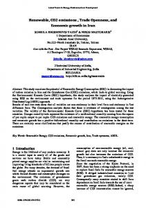
II. Trade openness At the time of the military coup, on 11th September 1973, import tariffs averaged 105% and were highly dispersed, with some goods subject to nominal tariffs of more than 700% and others fully exempted from import duties. In addition to tariffs, a lot of quantitative restrictions were applied, including outright import prohibitions, prior import deposits of up to 10.000% and a distortionary multiple exchange rate system consisting of fifteen different rates (De la Cuadra; Hachette 1991). The military government, under the economic guide of the so-called Chicagoboys, declared the purpose not only of restructuring the economic stability and of normalizing the relationship with the external creditors, but also of reversing the approach to the economic development of the socialist Allende. Between 1974 and 1979, the military government eliminated all the quantitative restrictions and gradually reduced nominal tariffs to an average and uniform value of 10%. Such average tariff value was extremely low for a developing country in the early 80s and a uniform tariff was uncommon also in the industrialized economies. Chile, with an astonishing rapidity, moved from an almost totally closed economy during the socialist government to one of the most open economies in the world. Figure 1 reports the liberalization index. This index summarizes five indicators in a numerical index ranging from 0 to 20, where zero indicates a totally closed economy and 20 stands for the maximum degree of openness. The five components are an index of import quotas, the ratio between the actual exchange rate and the nominal rate, the black market premium, an index of export quotas, and tariffs. (De la Cuadra Hachette 1991)1

1

For detailed information on the liberalization Index see section V.

3

Figure 1 Liberalization index 25

20

15

10

5

19 94

19 92

19 90

19 88

19 86

19 84

19 82

19 80

19 78

19 76

19 74

19 72

19 70

0

Source: De la Cuadra, Hachette, 1991

The liberalization index (Lib) assumes low values in the first years of the 70s, during the socialist government of president Allende (1970-1973), then shows a dramatic increase in 1974 and stabilizes in 1975 and 1976. At the end of the 70s the index increases significantly and then reaches the maximum degree of openness realized in the country in the first part of the 80s. With the debt crisis there was a little reversal, but during the second part of the 80s and the first half of the 90s the index grows. The liberalization program was associated with other policies: in particular, trade openness was sustained with an active policy on the exchange rate in order to maintain a competitive real rate. Trade openness resulted in a meaningful growth of non-traditional exports and imports. The radical changes in the structure and in the level of protection vigorously influenced the import composition. In particular, the trade openness process favored consumer goods, which were the more penalized before liberalization. It is remarkable that the consume of those goods, whose import was grown, was concentrated in the high-income classes of the population, increasing social differences. The export composition also radically changed. The manufacturing and agricultural exports increased, in particular in no-traditional sectors, and, on the contrary, natural resource exports fell. 4

In the first years of the 80s, because of the debt crisis, trade openness suffered a modest and temporary reversal. Between 1977 and 1981, Chile had been accumulating a huge amount of foreign debt: the main part was composed by loans, which was not guaranteed by the Government, granted by foreign banks to Chilean private firms. Until 1981, the net flows exceeded the absorbing capacity of the national economy, so international reserves accumulated and generated a pressure on the exchange rate. Since import growth exceeded the export increase, there was a persistent deficit of the balance of trade, covered with a huge capital flow. The supply excess of financing sustained the increase in the national expense and reduced the internal savings: as a result, the Chilean economy became increasingly dependent on foreign capital. When the debt crisis broke in 1982, the foreign capital flows fell dramatically, the interest rates grew significantly and trade terms worsened. To overcome the crisis, it was necessary to increase exports and contextually reduce imports. To do so tariffs were elevated to 35% and export subsidies were introduced, but no quantitative prohibitions were imposed. From 1985, after the crisis, tariffs started to decrease and this process continued until 2003, when tariffs reached the level of 6%. In the 90s changed the strategy of the commercial policy. From unilateral trade liberalization, Chile passed to a bilateral strategy based on reciprocal agreements. Trade policy transformed a dramatically closed economy in one of the most opened countries of the world. This process deeply transformed Chile and permitted an astonishing development. Anyway, a so deep transformation can influence several economic and social aspects of a society. This study analyses the impact of trade liberalization on the wage distribution in Chile. In particular, the main purpose is to test if the trade policy generated greater inequality in the country.

III. Wage distribution In the last 40 years, Chile experienced deep economic, social and political transformations that permitted a greater level of economic development, a higher growth rate and a meaningful poverty reduction. The same progress was not experienced in the wage distribution, which remains seriously unequal.

5

The matter of inequality is particularly relevant for a country like Chile: Latin America is one of the regions with higher levels of inequality and inside the region, Chile is one of the countries with the worst values. From the Great Depression, that strongly affected Chile, distributive conflicts intensified and several policies were implemented to reduce inequality, but the effect was a restriction of the economic activity without any meaningful impact on the wage distribution. Trade openness permitted the access of a greater number of consumers to a better and greater basket of commodities, but only a small fraction of population benefited of these improvements. In this section, the article analyses inequality in Chile from 1970 to 1995. In particular, the study focuses on the wage difference between workers that reached different educational levels as a proxy to estimate the skill premium.

III.1 Wage inequality (1970-1995) This section describes the inequality dynamics in the period 1970-1995. Data are from the Employment and Unemployment Survey for the Greater Santiago, realized by the Economics Department of Universidad de Chile2 First, two inequality indexes were calculated: this type of coefficients permits a quick overview of income distribution. Since we are interested in wage distribution, the coefficients have been calculated on a restricted sample. This sample includes only men which earn a wage and with a full-time job. Women are excluded to avoid biases in the analyses for two reasons: the female participation rate to the labor market varied a lot during the period considered and it is seriously correlated with the educational level. The two inequality indexes calculated are the Gini coefficient and the ratio between the 5th and the 1st quintile of the wage distribution (Q5/Q1). Calculating both is useful because of their different sensitivity to changes in the wage distribution: in particular, the Gini coefficient is more sensitive to movements in the middle of the distribution, and the ratio Q5/Q1 is more sensitive to the extreme values. Figure 2 shows the Gini coefficient calculated in the period 1970-1995.

2

For more information on the dataset see Annex 1.

6

The Gini coefficient increases from the middle of the 70s until 1987. The lowest values are in the period 1972-1973, during Allende’s socialist government. The maximum value is in 1987. The meaningful aspect of the figure is that inequality grew for almost all the period considered, in a country already characterized by high levels of inequality. From the value of 0,42 in 1974, the Gini coefficient increases to 0,58 in 1987, and, despite a decrease in the first years of the 90s, during the transition to democracy, the 1995 level is still higher than the ones experienced in the first half of the 70s.

Figure 2

Gini coefficient 0,6

0,55

0,5

0,45

0,4

19 94

19 92

19 90

19 88

19 86

19 84

19 82

19 80

19 78

19 76

19 74

19 72

19 70

0,35

Processed by the author from the Employment and Unemployment Survey for the Greater Santiago by Universidad de Chile

Another index that was calculated is the ratio Q5/Q1. In figure 3 there is the ratio Q5/Q1 calculated for the period 1970-1995.

7

Figure 3 Q5/Q1 SAL30

18 16 14 12 10 8

94 19

92 19

90 19

88 19

86 19

19

84

82 19

80 19

78 19

76 19

74 19

72 19

19

70

6


Analyzing the ratio between the 5th and the 1st quintiles of the wage distribution, we can observe that in the years of Allende’s government the ratio decreases. Starting from 1975 the ratio increases until the end of the 80s. In the first years of the 90s there is a reduction, probably due to the more attention paid to distributive problems by the Concertación de Partidos por la Democracia, the political coalition that guided the transition to democracy during the 90s.

The analysis of these inequality indexes tells us that, during trade liberalization, wage inequality increased in Chile, particularly between the intermediate classes and in the top part of the wage distribution. It is important to notice that the initial values of inequality were high. In 1970 the Gini coefficient was about 0,5 and the inter-quintile ratio was 11.

III.2 Wages and educational levels Inequality indexes are a valuable instrument to understand inequality but, in order to assess the effects of trade liberalization on the wage distribution, it is important to discriminate between skilled and unskilled labor. The educational level was used as a proxy of the individual skills.

8

Workers were divided in three classes according to the educational level reached and than the wage gap between different groups was calculated. The categories are three: - Elementary: in this group are classified workers that concluded the first educational level and workers with incomplete secondary education. This category includes people that studied between 8 and 11 years. - Secondary: in this group are classified workers with secondary education and individuals with incomplete university education. This category includes people that studied between 12 and 16 years. - University: this group includes workers that obtained a university degree. Two are the measures of the wage gap: the natural logarithm of the ratio between the average wages and the estimated skill premium.

III.2.1 Average wages The first gap measure is the ratio between the average wages. The wage gap is defined as the natural logarithm of the ratio between the average wages calculated for the different educational levels. Figure 4 displays the wage gap between workers with university studies and high school graduates (secondary education). Figure 4 Ratio between average wages (university/secondary education) 1,65 1,45 1,25 1,05 0,85 0,65 0,45

19 94

19 92

19 90

19 88

19 86

19 84

19 82

19 80

19 78

19 76

19 74

19 72

19 70

0,25


9

The wage gap between workers with university and secondary education decreases in the first half of the 70s, than increases almost continuously from 1974 to 1987. In the first part of the 90s there is a little decline, but the gap value is still wide. Figure 5 reports the natural logarithm of the ratio between university and primary- education average wages. The wage gap between workers with university and primary education declines in 1971-1972 and then increases from 1973 until the end of the 80s. In the first years of the 90s the gap decreases, but in 1995 there is a reversal.

Figure 5 Ratio between average wages (university/primary education) 2,2 2,1 2 1,9 1,8 1,7 1,6 1,5 1,4

19 94

19 92

19 90

19 88

19 86

19 84

19 82

19 80

19 78

19 76

19 74

19 72

19 70

1,3 1,2


Figure 6 reports the wage gap between workers with a secondary degree and workers with primary education, calculated as the natural logarithm of the ratio between the average wages.

10

Figure 6 Ratio between average wages (secondary/primary education) 1,2 1,1 1 0,9 0,8 0,7 0,6 0,5 0,4

19 94

19 92

19 90

19 88

19 86

19 84

19 82

19 80

19 78

19 76

19 74

19 72

19 70

0,3


In the period 1970-1995 the wage gap between workers with secondary and primary education decreases, with the exception of a peak in 1979. According to the indexes, wage inequality increases between workers with a university degree and workers with lower education. The gap between individuals with secondary education and workers that completed the primary school decreases in the same period. Therefore, the wage inequality dynamics is not the same for the different classes of workers. Inequality increases between workers that are more educated and declines between less educated ones.

III.2.2 The skill premium Another measure of the wage gap is the skill premium. It is defined as the positive wage difference perceived by a worker because of a higher educational level reached. This indicator is an estimate and has the aim of isolating the part of the wage difference due exclusively to an educational difference. In fact, average wages consider the gross difference between workers with different levels of education, but the wage gap can be influenced by factors independent from schooling. For this purpose, the

11

estimation of the skill premium controls for other variables that can generate wage discrepancies. The skill premia have been estimated using a Mincer type regression for each year between 1970 and 1995. Mincer (1974) affirms that the productivity of a worker, and then his income, is determined by the individual stock of human capital. This type of capital is obtained through formal education and informal education, i.e. the skills acquired working. An individual requires a higher wage to make a job that needs a longer period of training. The formation of human capital is considered like an investment, so higher investment requires higher returns. The additional remuneration due to a marginal increase of schooling is a good estimate of the return to education. The extension of the Mincer model consists in introducing a matrix of dummies indicating the educational level attained, instead of the years of schooling, in order to estimate the additional wage perceived by a worker with a higher educational level, and not only the return of a marginal increase in schooling. The equation, estimated with OLS for each year between 1970 and 19953, is: ln wi = β 0 + β 1 Exp i + β 2 Exp i + β 3 ExpEst i + β 4 X i + δ Di + ε i 2

where wi is the individual wage and Expi is the estimated experience. Experience 2

represents informal education and is calculated as age - years of schooling - 6. Expi is the square of experience. ExpEst is the interaction between experience and education. X is a matrix of other controls: it includes a dummy that says if an individual is head of household and a variable that indicates if the individual is a full time worker, i.e. he works more than 30 hours per week. D is the matrix of the dummies created according to the different educational groups defined: elementary, secondary and university. The dummies take value 1 for the educational level reached and 0 in the other cases. The skill premium is calculated as the difference between the estimated coefficients of the dummies. For example, the skill premium of a worker that reached a university degree respect to an individual with completed secondary education is the difference between the coefficient of the dummy “university” and the coefficient of the dummy “secondary”. 3

In Annex 2 the results of the regressions are reported.

12

The main problem in the estimation of a wage function is the omission of relevant variables. The individual wage could be determined not only by informal and formal education, but by other individual qualities too. If this omission error would be significant the OLS estimation would be biased. Several studies on this point demonstrate that this omission error, if it exists, is negligible. (Arellano and Braun 1999). Figure 7 shows the skill premium of a worker with a university degree respect to a worker with secondary education. The gap between workers with a university degree and individuals with a high school degree grows from 1974 until the end of the 80s. In the first half of the 90s there is a little decline, but the difference is still high.

Figure 7 Gap between university and secondary education 1,5 1,3 1,1 0,9 0,7 0,5 0,3

19 94

19 92

19 90

19 88

19 86

19 84

19 82

19 80

19 78

19 76

19 74

19 72

19 70

0,1


Figure 8 reports the estimated gap between university and elementary education.

13

Figure 8 Gap between university and elementary education 2 1,8 1,6 1,4 1,2 1 0,8 70 19

72 19

74 19

76 19

78 19

80 19

82 19

84 19

86 19

88 19

90 19

92 19

94 19


The gap between workers with university and elementary education grows from 1973 to the first half of the 80s, then, in the first years of the 90s decreases dramatically, but the 1995 value is still higher than that of the 70s. Figure 9 reports the gap between secondary and primary education.

Figure 9 Gap between secondary and elementary education 0,95 0,85 0,75 0,65 0,55 0,45 0,35

19 94

19 92

19 90

19 88

19 86

19 84

19 82

19 80

19 78

19 76

19 74

19 72

19 70

0,25


14

The gap between workers with secondary and primary education decreases during all the period, with the exception of 1979. This is the only gap decreasing, so it is very interesting to analyze if trade openness contributed to this reduction.

IV. Theory and empirical evidence The Heckscher-Ohlin model predicts, as a result of trade openness, an asymmetric dynamics of the wage gap between skilled and unskilled labor in developed and developing countries. The model considers two countries, a developed country and a developing one, two goods, and two factors of production, skilled and unskilled labor. In particular, the developing country is considered unskilled labor-abundant, so it has a comparative advantage in the unskilled labor-intensive good. On the contrary, the industrialized country is skill labor-abundant, and it has a comparative advantage in the skill-intensive good. When the countries liberalize, the Stolper - Samuelson theorem predicts that the return of the factor used intensively in the production of the good exported increases and the return of the factor used intensively in the production of the import-competing good declines. Therefore, the gap between skilled and unskilled labor widens in the developed country and it decreases in the developing one. However, several empirical studies highlight a symmetric dynamics of the wage gap between developed and developing countries, so the conventional framework fails in explaining growing inequality in the developing countries. It is necessary to refer to a model that introduces other hypotheses. In order to address the issue of the impact of globalization on wage inequality, it is useful to consider the factor-specific model of international trade. The possible social impact of trade openness depends on the way labor markets function and in particular on the degree of labor mobility. Following Jones (1971) and Jones and Engerman (1996) the factor-specific model allows a richer specification of wage dynamics respect to the conventional model. This is so because there is no longer a one-to-one relationship between wages and prices: in this model, prices are just one determinant of wage formation, and other meaningful factors are the biased technological change and labor supply changes.

15

This is particularly relevant for the case of Chile, a natural resource- abundant country. The model considers three factors of production: capital invested in natural resources, which earn r, skilled labor (LS), that receives a wage wS, and unskilled labor (LU) that earns a wage wU. Natural resources can be considered a specific factor in nature. In the labor market, certain rigidity is introduced: the unskilled labor is considered a specific factor, because the skills of this group are difficult to transfer between sectors and the shift requires a longer period. On the contrary, skilled labor is considered a mobile factor, because the skills of these workers can be easily transferred from a sector to another. The economy produces, with these three factors of production, two commodities X and Y. The good X, in the production, uses intensively natural resources, which are considered complementary to skilled labor. The good Y uses skilled and unskilled labor. Chile is supposed to have a comparative advantage in the natural resources-abundant good X, so this commodity is exported. When the country liberalizes, the price of the exported commodity X increases and the price of the import-competing good Y decreases. Therefore, the production of X grows and the production of Y falls. As a consequence, the return to natural resources, factor used intensively in the production of the exported good, grows. In the importcompeting sector Y prices and production decrease and the wage of unskilled workers declines. Some skilled workers will move from sector Y to sector X because of liberalization. The wage of skilled workers increases, but less than the return to capital invested in natural resources, because of the entry of some skilled workers from sector Y. Calling PX and PY the prices respectively of goods X and Y, we can summaries this as: rˆ > Pˆx > wˆ s > Pˆy > wˆ u Therefore, the variation of the specific factor return, in absolute value, is greater than the change in the mobile factor return. Trade openness makes natural resourceintensive goods more profitable, so the income distribution changes in favor of the owners of the resources. Moreover, certain groups of workers, in this case skilled workers, improve their wage position respect to other categories (unskilled workers). Therefore, this model shows that trade openness can generate increases in wage inequality in the developing countries when labor is not perfectly mobile.

16

As said above, technology is another relevant factor that affects wages. In the last decades we testified a meaningful technological development. A developing country is interested in innovating when it opens to international markets, to compete at the world level. Therefore, trade openness is undoubtedly a stimulus to introduce new technologies. A country can introduce new technologies through different channels: innovations can be created and produced in the country or they can be imported. Undoubtedly, the developed countries invest more on research and innovation and they can be considered as the principal innovators. So, in general, the developing countries tend to import new technologies from the industrialized countries. However, if new technologies are created in developed countries, rich of skilled labor, these innovations tend to substitute unskilled labor and to be complementary to skilled labor (Acemoglu 2000). Therefore, when these technologies are imported in a developing country, unskilled labor abundant, the effect can be a bias in the labor market, changing the composition of the demand of skilled and unskilled labor. If machinery requires more skilled workers, the demand of this type of labor increases and the wage gap raises, given labor supply. Because innovation enters in the developing country through trade liberalization, it can be considered as an indirect effect of trade openness on wage inequality. In the last decade, several studies were conducted to analyze wage inequality between skilled and unskilled workers, to discover the causes of a widening wage gap and to understand the role of trade liberalization. The main part of these studies evidences a growing wage gap and attributes this phenomenon to trade liberalization and skill-biased technological change. The empirical evidence on developing countries shows that, except for some Asian countries, the wage gap between skilled and unskilled workers increased after trade liberalization (Wood 1997). Robbins (1995) summarizes and compares some country studies conducted on Argentina, Chile, Colombia, Costa Rica, Malaysia, Mexico, Philippines, Taiwan and Uruguay, to test the Heckscher-Ohlin model. He uses data from household surveys and concludes that the HO predictions are inconsistent with the empirical evidence, because variations in labor supply influence relative wages between different groups of workers,

17

probably because of an isolation of the labor markets from the effect of the factor price equalization theorem. In Colombia wage inequality increased as demonstrated by Attanasio, Goldberg and Pavcnik (2002), who realized an empirical analysis of the relationship between wage distribution and trade openness. They use household surveys and a Mincer type equation to analyze the effects of liberalization on wages and relative labor supply. The commercial policy played a role, but the increase in the skill premium is mostly due to the technological innovation, that favored more skilled workers, generating a bias in the labor market. Nevertheless, this biased technological change is favored by trade openness, because lower tariffs permitted the entry of new technologies developed abroad, typically in developed countries. In conclusion, trade liberalization had an impact on the relative wages of workers with different levels of education, but other factors could have influenced income distribution. In Brazil too was implemented a program of trade liberalization and Pavcnik et al. (2002) study the effects of this policy on the wage distribution between skilled and unskilled workers. They conclude that the trade reform contributed to increasing inequality through a biased technological change induced by the liberalization. They do not find any type of support to Heckscher-Ohlin, in fact tariff changes seems not to be connected to factor occupation. Other studies on Latin America went to the same conclusions: trade openness had an impact on wage distribution, but in many cases the effect was small. Technological change played an important role and it can be considered as an indirect effect of trade liberalization, because the greater part of innovations is not created and produced in the developing countries, but is imported from the developed countries, through the import of capital goods and machinery or through foreign direct investments. Other studies were conducted on the peculiar Chilean case. Pavcnik (2000) examines whether investments and adoption of skilled biased technology have contributed to within industry skill upgrading using plant level data. Using parametric and semi parametric approaches, she finds a relationship between plant level measures of capital and investment, the use of imported materials, foreign technical assistance, patented technology and skill upgrading.

18

Beyer, Rojas and Vergara (2000) use cointegration techniques to assess the long period relationship between the skill premium, product prices, trade openness and factor endowment. They conclude that openness, measured as trade volume in percentage of GDP, contributed to wage inequality, but the effect was of small entity. The ILO report on Chile (1998), presented in the Conference on Social Dimension of Globalization, compares different sectors of Chilean economy and highlights that Chile is specialized in natural resource-intensive exports. This report considers the factor specific model: trade openness stimulates the demand of natural resource-intensive goods, and this benefits the owners of this factor of production and skilled workers, which are considered complementary to natural resources. On the contrary, the wages of unskilled workers in the import-competing sectors decrease. These theoretical predictions are confirmed by the empirical analysis. This study regresses the wage gap, measured as skilled premium and as the ratio between the quintiles of the distribution, on proxies of technological innovation, trade openness and relative supply. As a proxy of technological change a time trend is used, whose coefficient is significant in all the regressions estimated. This seems the main factor that affects wage inequality. Trade openness has an impact, but of small entity. Anyway, technological change is favored and permitted by trade liberalization, so it can be considered as an indirect effect of this policy.

V. Trade openness and wage inequality in Chile This section, referring to the factor-specific model as described in section IV, assesses the impact of trade openness on wage inequality between skilled and unskilled workers in Chile. To understand the effects of liberalization on the wage gap I performed a regression of the wage differential on some explicative variables. The regression estimated is: Skillpremi umt = α + β Openness t + χSupply t + Skillpremi umt −1 + ε t

The dependent variable is the skill premium as a proxy of wage inequality between different groups of workers. In section III, two measures of the wage gap were calculated: the logarithm of the ratio between average wages and the skill premium. The skill premium captures the net difference in wages due to the educational level, while

19

the ratio between the average wages is the gross difference, which can include the influence of some other characteristics of the individual. Since the two measures show a similar dynamics of the wage gap, in this part of the analysis we use the skill premium as a more accurate proxy for the wage gap between skilled and less skilled workers. In the regressions a measure of trade openness was introduced to estimate the impact of this variable on income inequality. To capture the effects of trade openness, two different proxies are alternatively used. The first indicator built is Open, which is the sum of exports and imports in percentage to GDP. This proxy is one of the most used in the empirical works that investigates the effects of trade liberalization, but it considers only the increase in the volumes of trade, which are not relevant in the conventional framework. Another proxy of trade openness is Lib, a more general liberalization index built by Professor Dominique Hachette of Universidad de Chile. This index summarizes five different aspects of liberalization in a numeric indicator ranging from 0 to 20. These indicators are: an index of import quotas; the ratio between the actual exchange rate and the nominal rate; the black market premium; an index of export quotas; and tariffs. The index of quantitative restrictions is based on an estimation of Ffrench-Davis (1973) to summarize the effects of prohibitions, quotas, administrative delays and so on. A monthly count of all the restrictions, in a numeric value, is transformed in an annual qualitative index ranging from 0, perfect-closed economy, and 20, opened economy. The second part of the Lib index is the ratio between the actual exchange rate and the nominal one. The nominal rate was estimated as an arithmetic average of exchange rates that prevailed in the reference period, with the adequate weight to the single different rates. To obtain the actual rate, they added the cost of preventive deposits and others to the nominal value tariffs actually paid as a percentage of total import. The third element of the index is the coefficient between the black market rate and the official rate. This is a good indicator to assess the rigidity of controls on the exchange market. The fourth component is not relevant for the period analyzed because export quotas were eliminated before 1970. The last component consists in tariffs.

20

Another variable introduced in the analysis is a proxy of relative supply (Supply) of skilled labor. The relative supply is calculated as the ratio between hours worked by each class of individuals, according to the educational level, using data from the Survey. The factor specific model and several studies on this topic highlight the importance of inserting a technological variable in the regression, but it is difficult to estimate the technological change induced by trade openness. The effect of this channel of innovation can be captured through an index of capital good imported as a percentage of GDP or through a time trend. To build a more precise index a more detailed dataset is needed. For the case of Chile, a dataset that reports plant-level detailed information exists, but it does not permit a discrimination of workers on the base of education. In fact, this dataset classifies workers only as blue collars or white collars. Since these variables are not precise in assessing the technological change, the article reports only the specification without the technological variable. The analysis is divided into two parts. The first part investigates the relationship between wage inequality and trade openness, considering the gap between workers with university degree and individuals that completed the high school, the second one analyzes the gap between workers with secondary and primary education.

V.1 Gap between workers with university and secondary education As seen in section III, this gap is increasing for almost all the period considered. The aim of the analysis is to assess the impact of trade openness on this growing gap. The regression estimated considers, as a dependent variable, the skill premium between workers with a university degree and individuals that completed the secondary education. The regression is estimated using data from 1970 and 1995 with OLS method. (Eq.1) skillpremiumLDt = α + β1 Libt + β 2 Opent + χSupplyt + φskillpremiumLD (t −1) + ε t

The proxies for trade liberalization are included alternatively in the equation.

21

In the regression is introduced, as an explicative variable, the dependent variable lagged of one period. There is a certain degree of inertia in the wage variation and in the wage gap too. Table 1 reports the estimated results. The numbers in the first row identifies the two different specifications, inserting alternatively the proxies for the trade liberalization process. All the variables are in logarithm, except the liberalization index (LIB). The numbers reported in brackets are the t statistics for the estimated coefficients. The stars after the estimated coefficients indicate if they are significant. Three stars indicate a coefficient significantly different from zero at a confidence level of 99%. Two stars stands for a confidence level of 95%, one star for 90%. The table also shows the F statistics, the R2 and the R2 adjusted.

Table 1 Skill premia 1 0,0179**

LIB Open

2 (2,24)

0,6832*** (3,70)

-0,4821***

-0,4962***

(-6,49)

(-5,68)

0,1407

0,2158*

(1,29)

(1,75)

-2,9520***

-0,8552***

(-4,66)

(-6,27)

F

35,449

24,845

R2

0,8351

0,7802

R2 adj.

0,8115

0,7488

Relative supply Yt-1 Constant

The coefficient of the relative supply is significantly different from zero and it is negative. This is the expected result: if the relative supply of workers with a university degree increases respect to the workers with a high-school degree, the wage of the first group of workers diminishes and the wage gap decreases.

22

The lagged dependent variable is not significant in the first specification, and significant in the second specification, with a confidence level of 90%. This variable captures the inertia in wage dynamics and in this case, we cannot conclude on the relationship between the skill premium and its lagged value. In first specification Open is the proxy for trade openness. This variable is significantly different from zero and it is positive. This means that if Open increases the dependent variable (skill premium) increases too. Trade liberalization contributes to then higher inequality between workers with a university degree and individuals with a high-school degree. In the second specification, the proxy for trade liberalization is the numerical index Lib, which considers several aspects of the liberalization process. In this case too, the estimated coefficient is significant and positive, so the second specification confirms that trade openness contributes to higher inequality between more educated workers. As trade liberalization has an influence on the growing gap, it is interesting to study whether it has the same influence on the decreasing gap between workers with secondary and primary education.

V.2 Gap between workers with secondary and primary education The most important analyses conducted on Chile concentrate on the growing gaps, and neglect the gap between secondary and primary education workers, which decreases in the period 1970-1995, but it is important to analyze the effects of trade openness in this case too. To do this, the same exercise of section V.1 was repeated, changing the dependent variable. The equation estimated considers as the dependent variable the estimated skill premium that receives a worker with a high-school degree respect a worker that only completed the primary school: (Eq.2) skillpremiumDEt = α + β 1 Libt + β 2 Opent + χSupplyt + φskillpremiumDE (t −1) + ε t

Table 2 reports the estimated results. The numbers in the first row identifies the two different specifications, inserting alternatively the proxies for the trade

23

liberalization process. All the variables are in logarithm, except the liberalization index (LIB). The numbers reported in brackets are the t statistics for the estimated coefficients. The stars after the estimated coefficients indicate if they are significant. Three stars indicate a coefficient significantly different from zero at a confidence level of 99%. Two stars stands for a confidence level of 95%, one star for 90%. The table also shows the F statistics, the R2 and the R2 adjusted.

Table 2 Skill premia 1 0,0032

LIB Open

2 (0,45)

-0,1692 (-0,70)

-0,1374

-0,1889**

(-1,43)

(-2,08)

0,5250**

0,6042***

(2,74)

(3,71)

0,2751

-0,3231**

(0,34)

(-2,20)

F

8,264

8,064

R2

0,5414

0,5353

R2 adj.

0,4759

0,4689

Relative supply Yt-1 Constant

The relative supply coefficient is negative, as expected, but significantly different from zero only in the second specification. Trade openness seems not to have an effect on the gap between these two groups of workers. In fact, in both specifications, none of the estimated coefficients of the trade proxies is significantly different from zero. The lagged dependent variable is significant in the two specifications. The results of the estimation of this equation tell us that more research is needed to understand the reduction of the wage gap between these two groups of workers. Trade openness does not have a significant effect on the wage gap, so it does not contribute to the reduction nor it stimulates the increase of the wage gap.

24

While trade contributes to widen the gap between workers with a university degree and with secondary education, it does not influence the gap between less skilled workers. Therefore, the dynamics of the wage differential between workers with secondary education and workers with primary education is due to other factors, and trade openness has a different impact on the wages of workers with different skill level.

VI. Conclusion In 1973 Chile started a deep program of trade liberalization. This study investigates the effects of trade openness on the wage distribution, using the educational level to discriminate between skilled and unskilled-labor. Section III analyses the wage distribution in Chile during the period 1970-1995: the wage gap between workers with university education and individuals with secondary education increased in the period, while the wage gap between individuals with secondary education and workers with primary education declined. Section V studies the effects of trade openness on these two gaps. In the first case, the wage gap increased, and from the regression analysis appears that trade liberalization contributed to its growth. The same exercise is conducted for the decreasing gap. If trade openness widens the wage gap between more educated people, but diminishes inequality between less educated workers, the total effects will be ambiguous. Studying the effects of trade openness on the wage gap between workers with secondary and primary education reveals that in this case trade liberalization has no effect; in fact the estimated coefficients of the proxies for trade liberalization are all not significantly different from zero. About technological innovation induced by trade the results are not clear and this aspect needs further analyses and more detailed data. In conclusion, trade openness provoked greater wage inequality in Chile, but only between more skilled workers.

25

Annex 1 Data This analysis uses data from the Employment and Unemployment Survey for the Greater Santiago, realized by Economics Department of Universidad de Chile. It covers a sample of approximately 4.000 households, corresponding approximately to 10.000 observations per year, located in the Greater Santiago area, which implies the absence of information about very meaningful economic activities such as farming, fishing and mining, and the consequent over-representation of the importance of manufacturing in the country’s economy. Despite the problem of coverage, this dataset has the strength that the collection methods remain the same for all the sample period and that it provides detailed information on wages and education. The data collected cover: demographic information, occupational information, educational information, and income information. Demographic information includes sex, age and relationship with the head of household. Occupational information includes industry, job activity and hours worked per week. Educational information includes educational level and years of schooling. The educational levels are four: primary, secondary, university and special. The income sources contemplated in the survey are: salaries and wages, revenues in kind and bonuses, revenues of independent activities, pensions and other revenues. These data give rise to the following variables: - Total Income from Work = Salaries and Wages + Revenues of Independent Activities - Individual Total Revenues = Revenues of the Work + Revenues in kind and bonuses + Pensions + Other Revenues - Total Household Income = Sum of the Total Revenues of the Household (Morone 2001) The sample was reduced to consider only men. Women are excluded to avoid biases in the analyses for two reasons: the female participation rate to the labor market 26

varied a lot during the period considered and it is seriously correlated with the educational level. The sample was further reduced to consider only men that earn a wage. In particular, the individual wage (w) is calculated as the individual total income from work only for workers classified as salaried. As a proxy of the skill level of the individual worker I use the educational level. Since it is difficult to classify a worker who attended a special school as skilled or unskilled, I eliminated the observations that classify the educational level as special. In particular, the dummy elementary includes people that studied between 8 and 11 years. The dummy secondary includes workers that studied between 12 and 16 years. The dummy university takes value 1 for people with more than 16 years of schooling. . Demographic and occupational information is used to build the other variable included in the regression to estimate the skill premia. The dummy full takes value 1 for individuals that declare to work more than 30 hours per week, so they are considered full time workers. The dummy jefe reports value 1 if the worker is classified as head of the household and 0 otherwise. The variable Exp is built as: age of the worker – years of schooling – 6. This is a proxy of the experience acquired working. The dataset does not report how many years an individual worked, so this is the best estimate we could perform. The number 6 represents the age at which people start to attend school. The variable Exp2 is calculated as the square of Exp. The variable EstExp is the interaction between the proxy for the job experience of the worker and his years of schooling. This sample is composed of an average of 1700 individuals per year.

27

Annex 2 Estimation of the skill premium (results of the regressions) ln wi = β 0 + β 1 Exp i + β 2 Exp i + β 3 ExpEst i + β 4 X i + δ Di + ε i 2

The table reports the estimation result of the Mincer-type regression to estimate skill premia.

Year 1970

Exp

1972

1973

(-7,91)

0,0004 (1,79)

8,2351 236,9 0,4941 (94,84)

-0,000

-0,040

0,5351

0,8185 0,3215 -0,501 0,00305 8,8308 174,2 0,4039

(-3,45)

(-0,29)

(-1,08)

(7,72)

0,0274 -0,0004 0,1696 (-6,31)

(3,99)

0,0291 -0,0005 0,1517 (-6,37)

(3,42)

0,0118 -0,0002 0,1339 (-3,05)

(3,02)

0,0144 -0,0003 0,1284 (-3,69)

(2,48)

0,0263 -0,0004 0,3337

-0,011

(-5,59)

(7,28)

-0,0001 -0,164 (-1,85)

(-4,56)

0,0197 -0,0041 0,1980 (-4,94)

(4,23)

0,0186 -0,0003 0,1888 (-3,90)

(3,65)

0,0200 -0,0003 0,1938 (-3,88)

(3,81)

0,0201 -0,0003 0,1475 (2,63)

1983

(6,29)

R2

-0,017

(3,18)

1982

(22,49)

F

(24,83)

(2,87)

1981

1,8325 0,2363 -0,579

(19,16)

cost

1,7989 0,2634 -0,753 0,00084 8,5493 340,0 0,5588

(3,41)

1980

1,0397

estexp

(20,53)

(-2,23)

1979

full

0,9893

(4,77)

1978

jefe

(8,39)

(2,40)

1977

Univer.

(-6,59)

(2,24)

1976

(8,27)

Secondary

(5,61)

(5,36)

1975

(-5,23)

0,0277 -0,0004 0,3339

(5,34)

1974

Elem.

0,0316 -0,0004 0,3500 (5,79)

1971

Exp2

(-3,39)

(2,43)

0,0144 -0,0003 0,1288 (1,95)

(-2,90)

(2,08)

(13,34)

(7,47)

(4,21)

(104,40)

(-6,44)

(16,73)

(101,05)

0,7533

1,3462 0,1849 -0,396

0,0007

7,7807 187,8 0,4110

(14,70)

(19,38)

0,6848

1,4390 0,3142 -0,745 0,00047 5,6721 147,7 0,4123

(12,45)

(16,98)

0,6403

1,4100 0,3283 -0,420

(11,99)

(16,78)

0,7528

1,5672 0,2114 -0,430 0,00144 3,0826 166,7 0,4536

(12,22)

(17,63)

0,8802

1,6630 0,2425 -0,453

(15,75)

(21,39)

0,7289

1,1603 0,3024 -0,400 0,00294 3,6902 226,2 0,4945

(11,22)

(17,78)

(-4,83)

(16,05)

(40,71)

0,8560

1,7847 0,2929 -0,567

0,0096

3,4579 259,6 0,5229

(14,88)

(22,17)

0,8239

1,7857 0,3117 -0,339

(12,88)

(19,88)

0,7823

1,6227 0,2734 -0,510

(12,79)

(18,06)

0,8413

1,7677 0,2938 -0,084 0,00117 0,8294 165,9 0,4698

(11,37)

(17,10)

0,7687

1,7449 0,3032 -0,098

(10,49)

(17,02)

28

(8,28)

(-10,71)

(5,15)

(8,17)

(8,35)

(4,67)

(6,18)

(7,51)

(7,69)

(7,65)

(6,82)

(6,49)

(6,78)

(4,90)

(-10,80)

(-5,69)

(-5,73)

(-6,82)

(-8,06)

(-3,76)

(-5,80)

(-1,18)

(-1,40)

(3,34)

(2,15)

0,0008 (3,65)

(5,82)

0,0009 (4,11)

(4,00)

0,0012 (4,33)

0,0007 (2,99)

(3,69)

0,0014 (4,51)

(84,87)

(66,73)

3,0029 145,9 0,3933 (33,03)

(31,29)

3,0757 219,9 0,4823 (35,88)

(38,27)

0,8593 205,2 0,4954 (7,82)

1,3009 165,7 0,4223 (12,16)

(7,82)

0,5059 173,9 0,4871 (4,84)

Year Exp Exp2 elem. 1984 0,0291 -0,0005 0,1977 (4,48)

1985

-0,004 (-0,59)

1989

-0,012 (-2,38)

1995

-0,0000 0,0487 (-0,13)

(0,80)

(-1,99)

(0,46)

(-4,14)

(1,08)

(-2,23)

(1,37)

(-1,46)

(1,22)

0,0052 -0,0002 0,0502 (0,89)

1994

(-0,33)

0,0011 -0,0001 0,0684 (0,21)

1993

(-1,95)

0,0096 -0,0002 0,0033 (1,60)

1992

(3,84)

0,0227 -0,0004 0,0761 (3,14)

1991

(-2,84)

0,0076 -0,0001 0,0301 (1,11)

1990

(2,69)

0,0031 -0,0001 -0,018 (0,47)

1988

(-6,54)

0,0200 -0,0002 0,2197 (2,99)

1987

(3,54)

0,0317 -0,0006 0,1466 (4,81)

1986

(-5,46)

(-2,35)

(0,82)

-0,0001 -0,118 (-1,26)

(-2,09)

0,0123 -0,0003 0,0583 (2,04)

(-3,03)

(0,96)

Second. 0,8199

Univer. jefe full 2,0054 0,2534 -0,203

(11,91)

(21,53)

0,7312

1,7704 0,1931 -0,174

(10,97)

(18,61)

0,8106

1,8498 0,2071 -0,166

(11,60)

(19,13)

0,5655

1,8143 0,2685 0,036

(8,13)

0,5360 (7,26)

0,5372 (6,93)

0,6146 (7,27)

0,6117 (8,69)

0,4619 (7,01)

0,4675 (6,47)

0,1523 (2,41)

0,4268 (5,98)

(19,41)

(6,14)

(4,72)

(5,07)

(6,41)

(-3,65)

(-2,95)

(-3,09)

(0,58)

1,7207 0,2428 -0,289 (17,15)

(5,83)

(-4,43)

1,6319 0,1863 -0,337 (15,91)

(4,71)

(-3,91)

1,8352 0,2884 -0,408 (16,85)

(7,01)

(-4,26)

1,8070 0,2220 -0,454 (19,63)

(5,88)

(-5,69)

1,4632 0,2172 -0,521 (16,43)

(5,97)

(-5,50)

1,3981 0,1814 -0,371 (15,23)

(4,88)

(-4,46)

estexp 0,0010 (3,42)

0,0013 (4,67)

0,0007 (2,47)

0,0018 (6,58)

0,0017 (6,16)

0,0013 (4,71)

0,0004 (1,19)

0,0007 (2,88)

0,0015 (6,61)

0,0012 (4,61)

cost F R2 0,4177 209,8 0,5122 (4,62)

0,2989 209,2 0,4976 (3,24)

0,3349 202,0 0,4978 (3,64)

0,3795 276,9 0,5683 (4,01)

0,7995 226,4 0,5170 (7,87)

0,9626 210,4 0,5023 (8,06)

0,9628 211,3 0,5116 (7,27)

1,1431 256,6 0,5462 (10,49)

1,3796 199,3 0,4866 (11,96)

1,4005 194,0 0,4753 (12,78)

1,1312 0,2539 -0,101

0,0022

1,4791 169,0 0,4570

(14,86)

(-0,83)

(10,66)

(10,69)

1,6805 0,2001 -0,397

0,0007

1,5035 209,1 0,5218

(17,95)

29

(6,53)

(5,22)

(-3,38)

(2,89)

(11,03)

References Acemoglu, Daron (2000) “Technical Change, Inequality and the Labor Market”, NBER Working Paper No. 7800. Arellano, M. Soledad; Matías Braun (1999). “Rentabilidad de la Educación Formal en Chile”, Cuadernos de Economìa, Año 36, No. 107, pp.685-724. Attanasio, Orazio; Nina Pavcnik; Pinelopi K. Goldberg. (2002) “Trade Reforms and Income Inequality in Colombia”, Prepared for the 2002 IMF conference. Beyer, Harald; Patricio Rojas; Rodrigo Vergara. (1999). “Apertura Comercial y Desigualdad Salarial en Chile”, Journal of Development Economics, Vol.59: 103-123. De la Cuadra, Sergio; Dominique Hachette; (1991) “Chile” Capitolo II, Vol.1 in “Liberalizing Foreign Trade” edited by D. Papageorgiou, M. Michaely, and A.M. Choksi, Cambridge, Massachussets. Ffrench-Davis, Ricardo; (2000); “Economic Reforms in Chile: from Dictatorship to Democracy”, the University of Michigan Press Ffrench-Davis, Ricardo; (2002) “Export Dynamism and Growth in Chile since the 1980s”, CEPAL Review, Vol. 76 Hachette, Dominique (1993) “Estrategia de globalización del comercio”, Estudios Públicos, No. 51. ILO (1998). “Chile” International Labor Office, Geneva Jones, Ronald W. (1971) “A three factor model in trade, theory and history” in: J.N. Bhagwati et al. (Eds.) “Trade, balance of payments and growth” North Holland, Amsterdam. Jones, Ronald W.; Stanley L. Engerman (1996). “Trade, technology and wages. A tale of two countries”, American Economic Review Vol.86: 35-40. Martínez, Javier.; Alvaro Dìaz; (1996) “Chile. The Great Transformation” The Brookings Institution Washington D.C. & the United Nations Research Institute for Social Development, Geneva. Mincer, Jacob (1974) “Progress in Human Capital Analysis of the Distribution of Earnings” NBER Working Paper No.53 Morone, Piergiuseppe (2002), “Globalization and inequality: the effect of trade liberalization on developing countries”, wp No. 42, SPRU, University of Sussex Pavcnik, Nina (2000a). “Trade Liberalization, Exit, and Productivity Improvements: Evidence from Chilean Plants” NBER Working Paper No. 7852. Pavcnik, Nina (2000b) “What Explains Skill Upgrading in Less Developed Countries?” NBER Working Paper No. 7846. Pavcnik, Nina; Andreas Blom; Pinelopi K. Goldberg; Norbert Schady. (2002). “Trade liberalization and labor market adjustment in Brazil”, Robbins, Donald J. (1995) “Trade, trade liberalization and inequality in Latin America and East Asia. Synthesis of seven country studies”

Working Paper, Harvard Institute of International

Development.

30

Robbins, Donald J. (1996) “HOS hits facts: facts win. Evidence on Trade and Wages in Developing World”, Working Paper, Harvard Institute of International Develpoment. Wood, Adrian (1995). “How Trade Hurt Unskilled Workers” The Journal of Economic Perspectives, Vol.9, No. 3: 57-80. Wood, Adrian (1997). “Openness and Wage Inequality in Developing Countries: The Latin American Challenge to East Asian Conventional Wisdom”, The World Bank Economic Review, Vol.11, No. 1: 33-57.

31