Page 1 ... Traffic lights signaling optimization consists in optimizing traffic-light cycle,. i.e, the of sequence of st
XIII Encontro Nacional de Inteligˆencia Artificial e Computacional
Traffic Lights Signaling Optimization as a Many-Objective Optimization Problem Saulo A. Matos1 , Andr´e B. Carvalho1 1
Departamento de Computac¸a˜ o – Universidade Federal de Sergipe (UFS) S˜ao Crist´ov˜ao – SE – Brasil
[email protected],
[email protected]
Abstract. These days different technologies are used in transport systems. In particular, there is an area that deals with the synchronization of traffic lights, where the main goal is to optimize measures found in traffic, usually correlated to the traffic flow, through the use of traffic simulators. Here, this problem is modelled as a Many-Objective Optimization Problem, optimizing six objective functions. For attaining this goal, a recent many-objective algorithm, NSGAIII, is adapted to problem. NSGA-III algorithm is evaluated through a series of experiments and compared to the multi-objective algorithm most explored in literature, NSGA-II. This set of experiments are conducted with the aid of a traffic simulator (SUMO).
1. Introduction The aim of Intelligent Transportation Systems (ITS) is to optimize transportation efficiency and to improve its safety through the use of technology. Such systems allow road users to be better informed and consequently make better trip-related decisions [Marcin et al. 2013]. The ITS technologies include different application spaces. One of them is traffic management, where efficiency can be increased by using new concepts of traffic organization and maintenance. As a basis for the process of influencing the traffic, adequate information on the current traffic situation has to be collected. Another important aspect of traffic management is to maintain a quality traffic flow. This means, in other words, to reduce congestion and travel time of vehicles. One way to obtain a quality traffic flow is through traffic light synchronization, ensuring a minimum waiting time, typically using optimization algorithms and a traffic simulator. The simulators were developed due to the growing demand for improved road traffic. With them, it is possible to make a local and global analysis of the traffic. The results generated by simulation can be useful to government entities in the risk analysis of of road networks in order to ensure maximum comfort and security to their users. A wellknown traffic simulator is SUMO (Simulation of Urban Mobility) [Daniel et al. 2006]. Traffic lights signaling optimization consists in optimizing traffic-light cycle, i.e, the of sequence of states (green, yellow, red) that a traffic signal iteratively runs [Javier et al. 2010]. In order to perform this optimization, simulators are used to model a traffic-light cycle. With the use of simulators, it is possible to represent different road intersections and traffic lights and to obtain several traffic quality measures like: travel and stopped time, number of vehicles that arrive at their destination, the overall average speed and traffic flow, carbon dioxide emission, among others. The solution is a
SBC ENIAC-2016
Recife - PE
421
XIII Encontro Nacional de Inteligˆencia Artificial e Computacional
vector representing the time of each phase for every traffic light in the simulation and the objective functions are the traffic quality measures. Since it is possible to use several objective functions, traffic lights signaling optimization is often modelled as a Multi-objective Optimization Problem (MOP) [Shen et al. 2013] [Javier et al. 2010] [Halina and Michal 2006]. MOPs involve the simultaneously optimization of two or more conflicting objectives functions subject to certain constraints. However, in spite of the existence of several quality measures, the majority of the related work often select a small set of objective functions (often two). Furthermore, these works often explores traditional multi-objective evolutionary algorithms (MOEA), like NSGA-II [Deb et al. 2002]. This limitation on the number of objective function lies on the incapacity of traditional MOEA to deals with a high number of objective function. These algorithms scale poorly when the number of objective functions increases (more than 3 objective functions) and face difficulties when the number of objective is greater than three [Ishibuchi et al. 2011]. These problems are called Many-Objective Optimization Problems (MaOPs). This paper has the goal to model traffic lights signaling optimization as a manyobjective optimization problem. Different from the related work, here six objective functions are used, namely: Depart delay, T rip duration, W ait steps (v < 0.1m/s), T ime loss (v < 60km/h), CO2 abs emitted and f uel abs consumption. The use o several objective function approximate the modeling of real situations through the use simulators, since it is important to consider different quality measures when defining trafficlight cycles. Furthermore, an algorithm specially designed to deal with MaOPs, NSGAIII [Deb and Jain 2014] is applied to the problem. To evaluate a the proposed approach, it is defined benchmarking using SUMO and different sets of experiments. The proposed benchmarking considers two different traffic simulations and two different traffic flows totalizing four scenarios. NSGA-III is compared to NSGA-II algorithm, which is the MOEAs used in the majority related work. The remainder of this paper is organized as follows: Section 2 presents the traffic lights signaling problem and Section 3 presents the basic concepts of many-objective optimization. In Section 4 is present the adaptation of NSGA-III to the studied problem. The benchmarking experiments and the discussion of the results are presented in Section 5. Finally, the conclusions and future works are discussed in Section 6.
2. Traffic Lights Signaling Optimization Synchronizing traffic lights is one of the approaches to reduce congestion problems in traffic. As a result, this task aspire to minimize some factors, such as traffic congestion, fuel consumption and the emission of gases (e.g. carbon dioxide carbon dioxide (CO2 ) and nitrogen oxides (NOx )). Synchronization is achieved when two or more traffic lights are running the same type of traffic signal plans in order to allow a vehicle to pass the traffic lights synchronized without stops. On the other hand, traffic signal optimization in general is a very complex problem, even for a single intersection can be no obvious optimal solution. The synchronization will not always ensure that vehicles will pass through open traffic lights. Good coordinated traffic signal plans are very hard to be created.
SBC ENIAC-2016
Recife - PE
422
XIII Encontro Nacional de Inteligˆencia Artificial e Computacional
The most important temporal quantities of traffic lights are the interval, cycle and phase. The interval is the time period in which all indications of traffic light remain static. Cycle is the succession of indications traffic light which repeat periodically. Phase is a part of the cycle devoted to a set of moves that are granted (or prohibited) the right pass simultaneously. In each phase is provided to vehicles a set of movements within the road. These movements may be entitled to pass through the intersection in the same direction, or performing conversion. Figure 1(a) [Shen et al. 2013] illustrates an intersection where there are six possible directions to go, but not all the directions are allowed at the same time. These directions are controlled by the phase sequence illustrated in Figure 1(b) [Shen et al. 2013].
(a)
(b)
Figure 1. (a) A 4 intersection road network. (b) Phase sequence of the traffic lights [Shen et al. 2013]
Given simulator and a combination of traffic lights, to model the traffic light synchronization as an optimization problem, three steps are necessary: to encode the traffic light scenario into a optimization vector (a solution); to decoded a possible solution into the representation adopted by the simulator; and, to execute the simulation and read the traffic quality measures. Therefore, it is possible to treat the traffic light synchronization problem as a combinatorial optimization problem representing possible combination of traffic lights though a vector. It is important to highlight that the construction of the scenario is achieved by the use of traffic simulators, such as SUMO. To model the traffic light synchronization problem as an optimization problem, it is necessary, given a combination of traffic lights, to build a computational representation of the duration of each phase for each traffic light. In this study, optimization occurred only for phases that have at least one direction receiving the green light. This implies that the phase where directions are formed only by red or yellow and red lights will have their time set at 4 seconds and will not be used in the optimization program. Thus, we can treat the traffic light synchronization problem as a combinatorial optimization problem by representing computationally a possible combination of the phase times of traffic lights through a vector. For the encoding/decoding process it is necessary to represent a possible set of intersection into a optimization vector. Figure 2 represents an optimization vector for a traffic network formed by two intersections with two traffic lights at each. In this scenario, with four traffic lights, it is possible to see the phases of each traffic light at each inter-
SBC ENIAC-2016
Recife - PE
423
XIII Encontro Nacional de Inteligˆencia Artificial e Computacional
section. The two colors (white and gray) separate the two intersections into two regions. At first, the phases are represented by the status of each traffic light during phases: green (G), yellow (Y) or red (R). Then, secondly, there is a representation of the duration, in integer, for each phase. This representation can be used in the optimization algorithm, where the duration of each phase is a finite set, usually with few options (ranging from four to one hundred). Therefore, this representation of the problem can be defined as a combinatorial optimization problem. All green phases of the network are arranged along this vector, which is the vector of solutions for the problem.
Figure 2. Solution encoding. Adapted from [Javier et al. 2010]
This process of representing a specific scenario into an optimization vector it is achieved by the use of the simulator. First the scenario must be designed into the simulator. For example, SUMO requires several input files that contain information about the traffic and the network to be simulated. It is necessary a file that represents the road network (net.xml). To generate it, also it is necessary to set up three more XML files. These three files represent: nodes (nod.xml), edges (edg.xml) and connections (con.xml) between the edges. The traffic lights are located on the nodes. Through the NETCONVERT module, it is possible to generate the road network. The process to generate the routes of vehicles is carried out through the DUAROUTER module, where a file (trips.xml) containing the flow of vehicles is used as input to generate another file (routes.xml) that will contain the routes of all vehicles. At this point, the only step left is to start the simulation and analyze the output files coming from SUMO itself, which have different quality measures for the various agents involved. Besides the vector representation, it is necessary a set of quality measures to be used as objective functions. For the optimization purpose, SUMO is used to evaluate a possible solution. Whenever a possible solution have to be evaluated, its vector representation must be decoded and used in the simulation. Every solution must execute a full simulation in SUMO: a solution represent the phase time for each intersection is decoded to the XML files; SUMO is executed according to the scenario configuration; after the simulation ends, all quality measures for the solution are presented into a XML file. It is possible to use several measures to optimize like delay time, stop time and travel time (average and total for all three types), the number of vehicles that arrive at their destination within a time interval, the overall average speed, traffic flow, fuel consumption and the emission of gases (e.g. carbon dioxide (CO2 ) and nitrogen oxides (NOx )), among others. Assuming that each vehicle will perform only one trip (origin node and destination node), for each simulation, each measure is calculated by the sum of the measure (m) obtained for each vehicle (v).
SBC ENIAC-2016
Recife - PE
424
XIII Encontro Nacional de Inteligˆencia Artificial e Computacional
1- Initialization
2- Generates New Solution
3- Decode Solution and Starts Simulation
4- Encode Solution and Optimizes Quality Measures Figure 3. Schematic representation of traffic lights signaling optimization
The traffic lights signaling optimization is summarized in Figure 3. The main steps are: initialization, generations of solutions, decoding and encoding process and optimization of the quality measures. Initialization: in this phase it is defined the network data and its characteristics (traffic lights and flow information). The information about the traffic scenarios are used to defined the parameters of the solutions such as, number of variables and interval range. With this data, it is possible to create an initial solution (often randomly), respecting the limit imposed by the network. Generates New Solution: through different search mechanisms, the optimization algorithm generates a new solution. The solution is a vector with the same length as the amount of green phases contained in the network. Decode Solution and Starts Simulation: after the generation of a solution, it is necessary to measure its quality. In this module, the values of the solution vector are decoded and then distributed among the existing traffic lights. This distribution consists of the updating of the duration values of green phases of these traffic lights. The traffic lights (phases and their durations) are on the same network file (net.xml). Now, with the updated values, the simulation starts. Encode Solution and Optimize Quality Measures: this phase extracts the quality measures previously established. The measures are extracted from the “trips.xml” file and inserted into a objective vector. 2.1. Related Works The combination of simulation and optimization algorithms to solve the traffic light synchronization problem is not new. Currently, a number of studies in the literature explores this approach. In [Shen et al. 2013], it was used NSGA-II algorithm to solve the traffic light signaling optimization problem with two objective functions: the average delay time and the average stop times. Furthermore, GPU programming and Cellular-Automata were used for the simulation and optimization system. Work [Halina and Michal 2006] proposes a signal optimization method based on a genetic algorithm supported by the microscopic simulation program. It aims at the minimization of time losses during the trip and maximization of average vehicles speed
SBC ENIAC-2016
Recife - PE
425
XIII Encontro Nacional de Inteligˆencia Artificial e Computacional
during the trip. The work uses detectors inside traffic network, thus leading to even more accurate results without significantly increasing computation time. In both settings used, good traffic conditions were achieved, with cars in constant motion, even where there are traffic jams. Queues at each entrance were quickly emptied and there were no situations where vehicles were not able to enter the study area. In the work of Javier et al. [Javier et al. 2010] a new model for traffic signal optimization was developed and tested based on the combination of three key techniques: 1) genetic algorithms for the optimization task; 2) cellular-automata-based traffic simulators for evaluating every possible solution for traffic-light programming times; and 3) a Beowulf Cluster. In the experiments four fitness functions were explored: number of vehicles that reached their destination (NoV), mean travel time (MTT), global mean speed, and TOC/SOC (TS, time of occupancy and state of occupancy). However, the problem was not modelled as multi-objective, and each measures were considered separately. In [Ali and Rahim 2015], through a genetic algorithm (encoded “Gray code”) and CORSIM simulator, the authors developed a meta-heuristics called IDSTOP. They incorporated microscopic models of traffic flow and attribute the volume of traffic. As a result, optimized solutions were achieved for the signal-timing parameters, and simultaneously the ideal traffic flow was defined. In spite of the possibility to have several quality measure, as far as we known, none of the previous related work explored more than four objective function simultaneously. In related work, authors selected a small sub-set of the quality measure or treated each function singly. Furthermore, these work did not explore techniques to deal with manyobjective problems.
3. Many-Objective Recently, several studies have shown that MOEAs scale poorly in many-objective optimization problems [Ishibuchi et al. 2011]. The main reason for this scaling property is that the number of non-dominated solutions increases exponentially with the number of objectives. The following consequences occur: first, the search ability deteriorates because it is not possible to impose preferences for selection purposes. Second, the number of solutions that are required for approximating the entire Pareto front increases. Recently, researches are using preference information, usually through a set of reference points. In [Deb and Jain 2014], it is proposed a reference-point-based manyobjective algorithm, called NSGA-III, that emphasizes non-dominated points that are close to set of reference points. These reference points are structured in a systematic approach of a normalized hyperplane presented by Das and Dennis [Das and Dennis 1998]. The paper concluded that the new approach was able to find a well-converged and welldiversified set of solutions. Another approach that achieves good results in MAoPs is the use of decomposition strategies [Bezerra et al. 2015]. Also, it is possible to explore specific characteristics of MOEAs to enhance their performance in Many-Objective Optimization. Here, this work will explore NSGA-III algorithm applied to a many-objective traffic lights signaling optimization problem.
SBC ENIAC-2016
Recife - PE
426
XIII Encontro Nacional de Inteligˆencia Artificial e Computacional
4. NSGA-III Applied to Traffic Light Synchronization Evolutionary multi-objective optimization algorithms demonstrated success in many practical problems involving mainly two or three objective functions. However, there is a growing need to develop evolutionary multi-objective optimization algorithms for dealing with many-objective problems [Deb and Jain 2014]. Given this, recently it was proposed a new version of the NSGA algorithm, now using a set of reference points for solving many-objective problems. The Non-dominated Sorting Genetic Algorithm III, NSGA-III, emphasizes population members that are non-dominated, yet close to a set of supplied reference points. The basic framework of NSGA-III is similar to the original NSGA-II algorithm with significant changes in its selection operator. But, unlike in NSGA-II, the maintenance of diversity among population members in NSGA-III is aided by supplying and adaptively updating a number of well-spread reference points. NSGA-III uses a predefined set of reference points to ensure diversity in obtained solutions. The chosen reference points can either be predefined in a structured manner or supplied preferentially by the user. In the absence of any preference information, any predefined structured placement of reference points can be adopted [Deb and Jain 2014]. In Section 2 we showed the traffic lights signaling problem and how to represent computationally the times of the phases of the traffic light in a vector. Once with a vector in hand we can use an optimization algorithm to define the times. Because it is a Many-Objective Optimization Problem, the NSGA-III is used to optimize six objective functions. An individual in NSGA-III represents a traffic light time plan. The fitness functions of each individual are defined by the simulator, as discussed before. Here a individual is defined as a integer array. As in NSGA-II, the NSGA-III algorithm does not require setting any new parameter other than the usual GA parameters such as the population size, termination parameter, crossover and mutation probabilities, and their associated parameters. The number of reference points H is not an algorithmic parameter, as this is directly related to the desired number of trade-off points. The population size N is dependent on H, as N ≈ H. The location of the reference points is similarly dependent on the preference information that the user is interested to achieve in the obtained solutions. The main steps of NSGA-III : first the population is initialized; every new solution must be evaluated through the execution of the simulator and after the evolutionary loop begins. In this loop, first is performed the Recombination+Mutation procedure to generate the offspring. Since the solutions are integer array, any basic evolutionary operator can be applied (step two from Figure 3). Every new solution must be evaluated (again by running the simulation, as in step three from Figure 3). Finally, the algorithm must define the new population based on the parents and offspring. Just like NSGA-II, the fast-nondominated-sort algorithm is performed to defined the new population. NSGA-III differ from NSGA-II by the crowding operator. In NSGA-III, the selection process based on the set of reference points is formed by three procedures, normalization, association and Niche-preservation [Deb and Jain 2014]. This process represents step 4 in Figure 3 and after the selection the evolutionary continues until a stop criteria is reached.
SBC ENIAC-2016
Recife - PE
427
XIII Encontro Nacional de Inteligˆencia Artificial e Computacional
5. Experiments This section describes the scenarios used in the experiment, the benchmark, further details of the simulator and the results. We tested two algorithms in two scenarios, with two traffic flows each. Each scenario is represented by a network and two flows (demands) of vehicles: low and high. In this study, two scenarios were defined. For each scenario, through the jMetal framework [Durillo and Nebro 2011], two algorithms were used and subsequently compared. The algorithms used were NSGA-II and NSGA-III. 5.1. Benchmark To perform the experiments some traffic flow scenarios are defined. To measure the performance of the algorithms in a many-objective problem different configurations were proposed. The main parameters are the traffic network (number of intersections) and the traffic flow (number of cars that pass through the network during the execution). Here, it is defined two networks, namely Scenario 01 and Scenario 02. Two different traffic flows were also defined, namely low and high flow. These parameters make up four different configurations defined by: • Scenario 01: This scenario (Figure 4(b)) is made up of 01 intersection and 04 injectors. For low flow, 3000 vehicles were used, and 21000 for high flow. In this scenario, with a high flow, each simulation took about 7 seconds. The encoded optimization vector has length two. • Scenario 02: This scenario (Figure 4(c)) is made up of 04 intersections and 08 injectors. For low flow, 6000 vehicles were used, and 42000 for the high flow. In this scenario, with a high flow, each simulation took about 19.8 seconds. The encoded optimization vector has length eight.
(a) Phases of all intersections in the experiments Network
(b) Scenario 01 Network
(c) Scenario 02 Network
Figure 4. Benchmark scenarios
Each one of the configurations share some parameters: it must be defined the flow of vehicles, number of roads, number of phases and interval of the phase. The flow of vehicles is previously defined and distributed randomly through the injectors. In this work, the injectors are all the nodes that are located on the network ends (injectors are numbered in Figure 4(b) and Figure 4(c)). In all scenarios, the number of injectors is twice the number of roads. The roads are two-way, where each road has six lanes, three for each way. The phases are also the same in all intersections. In SUMO,
SBC ENIAC-2016
Recife - PE
428
XIII Encontro Nacional de Inteligˆencia Artificial e Computacional
configuring a network in which intersections have a larger number of phases, or a different number of phases between the other intersections, does not constitute an increase in configuration complexity. However, it requires more time during configuration. And, as in this study, the number of phases is not the focus of the experiments, it was decided to maintain a simpler configuration. The Figure 4(a) below represents the phases of all intersections used in all experiments. In this study, a threshold was established contained in the interval: lower (l) and upper (u) of duration (d) of the green phases, where: (l, u) = {d ∈ N | 20 ≤ d ≤ 100} Other important feature of the benchmark is the objective function. Here, 6 different measures were used. The measures used in this work were: • • • • • •
Depart delay: The time the vehicle had to wait before it could start his journey; T rip duration: The time the vehicle needed to accomplish the route; W ait steps: The number of steps in which the vehicle speed was below 0.1m/s; T ime loss: The time lost due to driving below the ideal speed (60km/h); CO2 abs: The complete amount of CO2 emitted by the vehicle during the trip; F uel abs: The complete amount of fuel the vehicle used during the trip.
5.2. Algorithm Parameters The NSGA-III algorithm were compared to the main multi-objective algorithm used in the related work NSGA-II. Both algorithms were executed through the jMetal framework. It was used the default algorithms parameters defined by the framework. The parameters for NSGAs are shown in Table 1. Algorithm NSGA-II NSGA-III
Population Size 100 56
Table 1. Algorithm Parameters
Crossover Prob. 0.9 0.9
Mutation Prob. 1.0/Variables 1.0/Variables
Crossover Distrib. Index 20 30
Mutation Distrib. Index 20 20
In all scenarios (regardless of the traffic flow), for each of the two algorithms, 10 runs were executed. The total of objective function evaluation executed by each algorithm was 25200. This represents 25200 simulations each were done, totaling 252000 simulations per algorithm, or 504000 simulations per experiment in a given scenario (low or high traffic flow). In the low-flow experiments, each simulation has less than 1 second of duration. When the traffic flow is high, each simulation took about 8.3 and 19.8 seconds for Scenarios 01 and 02, respectively. In order to evaluate the performance of multi-objective algorithms quality indicators are used. These indicators are defined as functions that map sets of solutions to a real number. The hypervolume is a maximization metric that determines the area covered by the approximated Pareto front, which is created by combining the best values found for each objective. It is a common measure used in works where multi-objective algorithms are compared. In order to compare the performance of the algorithms we calculate the hypervolume, by considering a nadir point. In this experiment, the nadir was obtained all values executions.
SBC ENIAC-2016
Recife - PE
429
XIII Encontro Nacional de Inteligˆencia Artificial e Computacional
To measure the significance difference in each comparison, the Wilcoxon test is applied at 5% significance level. The test is applied to the hypervolumes. The Wilcoxon test indicates if there is any statistically difference between each analyzed data set and then, the average values are used to identify which algorithm has the best values. 5.3. Results Observing Table 2, each row represents a scenario and a traffic flow. The following values found in each scenario are displayed : the mean and standard deviation (between brackets) of hypervolume and the P -value obtained by Wilcoxon test. In all scenarios NSGA-II had the best results, because had higher values of mean of hypervolume. It is also noticeable (in the last column), through the P -value, that there is statistical difference in the first three experiments, because P -value < 0.05. However, in the last experiment (Scenario 02 with high traffic flow), there is no statistical difference, because P -value > 0.05. In both Scenarios, when the flow increases, the difference between the averages of hypervolume reduces. Table 2. Mean values of Hypervolume, Standard Deviation (between brackets) and P-value Scenario (Traffic Flow) 01 (low) 01 (high) 02 (low) 02 (high)
NSGA-II 2.58x10¹⁴ (3.23x10¹³ ) 1.83x1028 (4.06x1026 ) 6.73x10¹⁷ (1.97x10¹⁷ ) 4.95x1033 (9.27x1032 )
NSGA-III 1.19x10¹⁴ (4.31x10¹³ ) 1.04x1028 (1.34x1027 ) 1.24x10¹⁷ (1.98x10¹⁷ ) 4.06x1033 (1.04x1033 )
P-value 1.016x10⁻¹⁰ 1.083x10⁻⁵ 0.0001299 0.05243
Table 3 presents the average values of all objective functions of all non-dominated solutions found for both algorithms. In this table two measures had their scale changed for better visualization of the data, as follows: the depart delay calculated in hours (previously in seconds) and CO2 abs calculated in kilograms (previously in milligram). The other measures have their quantities as follows: duration (seconds), wait steps (integer), time loss (seconds) and f uel abs (milliliter). This analysis is performed to make a more detailed discussion of these results. Some measures had very similar results for both NSGAs, but for some the result was very different (with the defeated NSGA-III) and this was decisive in the calculation of the hypervolume. In two measures, the average value was very similar for both NSGAs, and in these cases NSGA-III always had the best values for these measures, as follows: CO2 abs and f uel abs. However, when the NSGA-II won, the difference between the average values when compared to NSGA-III was large, this occurred for two measures: duration and wait steps. Finally, the NSGA-II also won (or tied), but with a small margin when the compared measure was depart delay, except for the last experiment, where the NSGA-III had a small advantage. For scenarios with low traffic flow, the depart delay is close to zero, because there were few vehicles that had this delay. Regarding the lowest values found for the measures in all runs, it is worth highlighting some scenarios where NSGA-III had such values, wich were: Scenario 01 (low traffic flow) obtained lower values for all measures, except depart delay (tie). Scenario 02 (low traffic flow) had lower CO2 abs and f uel abs values. Finally, Scenario 02 (high traffic flow) had lower depart delay, CO2 abs and f uel abs values.
SBC ENIAC-2016
Recife - PE
430
XIII Encontro Nacional de Inteligˆencia Artificial e Computacional
Measures depart delay duration wait steps time loss CO2 abs fuel abs
Table 3. Average Measures
NSGA-II
Scenario 01 Low High 0.000305 23130 68225.3 706448 17602.9 294097 46984.9 557717 3561.82 23511.2 1420044 9373561
Scenario 02 Low High 0.00087 46286 179731 2171638 51589.1 880583 117205 1733454 7829.68 52499 3121578 20930589
NSGA-III Scenario 01 Scenario 02 Low High Low High 0.000305 23429 0.00087 46241 92126.0 880918 269466 2256486 40807.3 463116 128920 1065175 70864.0 732080 206939 1818322 3529.04 23267.0 7822.10 50989 1406974 9276201 3118553 20328895
In studies in the literature, the NSGA-III surpasses NSGA-II in problems with many objectives, but in this particular case (for the benchmark used in all scenarios), it did not. Given that it was expected that NSGA-III should not have been defeated by the NSGA-II, some hypotheses were raised with respect to why it occurred. The hypotheses are: the points of reference (which is very important in NSGA-III) may be somehow affected due to the great differences between values and quantities of the objectives. Another possible problem could be in the construction of solutions with integers within a small range and an also small vector, resulting in a very small search space. For the problem of reference points, it happens that the NSGA-III is using jMetal default values and this may not apply very well to the problem under study. Thus, the best would be to inform the reference points to the NSGA-III, as they are 6 measures and these measures have very large values, a more adequate choice of reference points would better guide the algorithm. Finally, for the issue of the search space, the first step is to use a binary coding, that would increase the size of the range and therefore the search space. Furthermore, we aim to insert a module for choosing viable solutions for each scenario and flows, where they will serve as the initial cutoff parameter for each solution generated by the algorithm. The need for this module arose when we observed that very bad solutions were found, especially at the beginning of executions. This happened for two reasons: the use of phase time values from random solutions, and because there were certain values that should never have been used.
6. Conclusion and Future Research In this study, we applied the NSGA-II and NSGA-III to solve a problem with six optimization objective functions. The six objectives are each of the summations (each vehicle) for each measure, they are: T rip duration, Depart delay, W ait steps (v < 0.1m/s), T ime loss (v < 60km/h), CO2 emitted and f uel used. We tested the methods on a network with 1 intersection and with 4 intersections in a hypothetical region. The experiments showed that NSGA-II outperformed NSGA-III for the given problem. In future works, we plan to use a binary encoding for phase times on both algorithms. We also intend to use more conflicting objectives, while joining linearly correlated measures in a single objective, for example certain emissions such as CO e NOx . In addition, as a way to reduce the number of objectives, we shall explore other techniques, such as dimensionality reduction. We also aimed to reduce the total number of vehicles, focusing on traffic situations with much shorter duration, however, maintaining the characteristics of intersections similar those used in this work. Thus, it is possible to drastically reduce the simulation time and thus enable a greater number of executions and more scenarios. That would allow for an increased benchmark.
SBC ENIAC-2016
Recife - PE
431
XIII Encontro Nacional de Inteligˆencia Artificial e Computacional
References Ali, H. and Rahim, F. (2015). A Program for Simultaneous Network Signal Timing Optimization and Traffic Assignment. In IEEE TRANSACTIONS ON INTELLIGENT TRANSPORTATION SYSTEMS, pages 1–6. IEEE. Bezerra, L. C., L´opez-Ib´an˜ ez, M., and St¨utzle, T. (2015). Comparing decompositionbased and automatically component-wise designed multi-objective evolutionary algorithms. In Gaspar-Cunha, A., Henggeler Antunes, C., and Coello, C. C., editors, Evolutionary Multi-Criterion Optimization, volume 9018 of Lecture Notes in Computer Science, pages 396–410. Springer International Publishing. Daniel, K., Michael, B., and Peter, W. (2006). The open source traffic simulation package SUMO. In RoboCup 2006 Infrastructure Simulation Competition, German Aerospace Centre, Institute of Transportation Research. IEEE. Das, I. and Dennis, J. (1998). Normal-boundary intersection: A new method for generating the pareto surface in nonlinear multicriteria optimization problems. SIAM Journal of Optimization, 8(3):631–657. Deb, K. and Jain, H. (2014). An Evolutionary Many-Objective Optimization Algorithm Using Reference-Point-Based Nondominated Sorting Approach, Part I: Solving Problems With Box Constraints. In IEEE TRANSACTIONS ON EVOLUTIONARY COMPUTATION, VOL. 18, NO. 4, AUGUST 2014. IEEE. Deb, K., Pratap, A., Agarwal, S., and Meyarivan, T. (2002). A fast and elitist multiobjective genetic algorithm: NSGA-II. IEEE Transactions on Evolutionary Computation, 6(2):182–197. Durillo, J. J. and Nebro, A. J. (2011). jmetal: A java framework for multi-objective optimization. Advances in Engineering Software, 42(10):760 – 771. Halina, K. and Michal, S. (2006). Genetic Approach to Optimize Traffic Flow by Timing Plan Manipulation. In Proceedings of the Sixth International Conference on Intelligent Systems Design and Applications (ISDA’06), pages 1–6. IEEE. Ishibuchi, H., Akedo, N., Ohyanagi, H., and Nojima, Y. (2011). Behavior of emo algorithms on many-objective optimization problems with correlated objectives. In Evolutionary Computation (CEC), 2011 IEEE Congress on, pages 1465 –1472. Javier, J., Manuel, J., and Enrique, R. (2010). Traffic Signal Optimization in “La Almozara” District in Saragossa Under Congestion Conditions, Using Genetic Algorithms, Traffic Microsimulation, and Cluster Computing. In IEEE TRANSACTIONS ON INTELLIGENT TRANSPORTATION SYSTEMS, VOL. 11, NO. 1, MARCH 2010, pages 1–6. IEEE. Marcin, S., Wojciech, M., and Djamel, K. (2013). Multi-Segment Green Light Optimal Speed Advisory. In Parallel and Distributed Processing Symposium Workshops & PhD Forum (IPDPSW), 2013 IEEE 27th International, pages 459–465. IEEE. Shen, Z., Wang, K., and F.-Y., W. (2013). GPU based Non-dominated Sorting Genetic Algorithm-II for Multi-objective Traffic Light Signaling Optimization with Agent Based Modeling. In Proceedings of the 16th International IEEE Annual Conference on Intelligent Transportation Systems (ITSC 2013). IEEE.
SBC ENIAC-2016
Recife - PE
432