Recent Advances in Intelligent Information Systems ISBN 978-83-60434-59-8, pages 641–653
Traffic Simulation Framework — a Cellular Automaton-Based Tool for Simulating and Investigating Real City Traffic Pawel G´ora University of Warsaw, Faculty of Mathematics, Informatics and Mechanics ul. Banacha 2, 02-097 Warszawa, Poland
[email protected]
Abstract Over the last century the number of vehicles engaged in the road traffic have been increasing rapidly. Traffic congestion and traffic jams became a serious problem, especially in big agglomerations. Various concepts are being applied to better understand the traffic flow phenomenon. In the paper we present the Traffic Simulation Framework (TSF) which is an information system for simulating a vehicular traffic in the real city road networks. The system is equipped with a comprehensive visualization which enables users to set and modify simulation parameteres and road network preferences. It also supports gathering detailed data related with the simulated traffic. In the paper we also describe a general traffic simulation model implementated a core module of the TSF system. It is a probabilistic cellular automaton model which is a strong generalization of some popular traffic simulation models. Keywords: traffic simulation, cellular automaton, multiagent systems
1 Introduction Vehicular traffic is a complex phenomenon. Over many years various methods from physics were applied to better describe and understand the traffic flow. Some interesting results were obtained by adopting methods from Newton’s mechanics, fluid dynamics, statistical mechanics and kinetic theory of gases (Schadschneider, 2000). They give better understanding of some fundamental aspects, but don’t take into account local correlations between vehicles and are unable to predict evolution of the real traffic precisely. A significant progress in the field was made by introducing models based on the cellular automaton theory. The most important of them is the NagelSchreckenberg model (Nagel, 1992) which have been extensively studied and generalized (Biham, 1992), (Chowdhury, 1999), (Schadschneider, 1999). It provides satisfactory results only in case of traffic on single-lane highways, but nowadays it is a fundament of many traffic simulation models. The model was also generalized and implemented in the Traffic Simulation Framework (TSF).
642
Pawel G´ ora
The intention of the TSF is to simulate real vehicular traffic in the city. The TSF is able to emulate motion of about 106 vehicles in the real-time1 on the real road network. The word “Framework” in its name is expedient, because the system gives opportunity to set, modify and test many parameters which may considerably change a characteristic of simulated traffic. The simulation model takes into account e.g., traffic signals, distribution of start point and destination points, various profiles of drivers and other parameters. The TSF makes it possible to specify simulation parameters in order to test their sensitivity and different simulation assumptions. In this paper we describe theoretical foundations of the TSF model and point out the most important features of the TSF, its possible applications and extensions. In Section 2 we present theoretical aspects of the TSF model, its mathematical background and assumptions. Section 3 introduces the TSF system which is a computer program developed by the author based on the TSF model. We discuss some interesting applications of the TSF in Section 4 and its possible extentions in Section 5. Finally, Section 6 concludes the paper.
2 Theoretical foundations of the TSF model The TSF model is a probabilistic cellular automaton which inherits some foundations from well-known Nagel-Schreckenberg model (NaSch model), introduced in 1992. First, we describe the most important aspects of the NaSch model. 2.1 Nagel-Schreckenberg model The NaSch model emulates a single-lane traffic. The road is represented as a tape divided into cells. Space, time and velocities are discrete. All cells have the same size (usually taken to be 7.5m). At any moment each cell may be empty or occupied by a single vehicle. The state of a single cell is just a velocity of the car which occupies the cell (or null if is cell is empty). This velocity of car i (denoted as vi ) is also considered as an internal state of car i and may take a value from the finite set {0, 1, ..., vmax }, where vmax is common to all cars (usually taken to be vmax = 5). The state of the automaton at time t + 1 is obtained from the state at time t by applying at the same time the following 4 rules to all cars: 1. Acceleration: vi (t + 1) := min(vi (t) + 1, vmax ) 2. Braking: vi (t + 1) := min(vi (t + 1), di (t)), where di (t) =number of empty cells in front of the car 3. Randomness: with probability p: vi (t + 1) := max(0, vi (t + 1) − 1) 4. Movement: car i moves forward vi (t + 1) cells. The first step models the assumption that every driver would like to drive as fast as possible. The second step indicates that drivers reduce the vehicle’s speed in order to avoid crashes (it is impossible to overtake, since the road has only one lane). The third step introduces a randomization to the model. It simulates that 1 machine:
Acer TravelMate 2482NWXMi, processor: 1,6GHz, RAM memory: 1,5GB
Traffic Simulation Framework
643
drivers sometimes spontaneusly reduce the vehicle’s speed due to e.g. weather conditions or psychological aspects. The fourth step is an actual motion of the car. All steps are crucial and cannot be removed to keep conformity to real vehicular traffic on highways. The experiments with computer simulations showed that NaSch model is able to simulate the real single-lane highway traffic with satisfactory precision (Nagel, 1992). It doesn’t give appropriate results in case of city traffic, where many more factors influence the traffic and driver’s behaviour. However, foundations of the model exists in most professional traffic simulation systems. 2.2 TSF model In this section we present the traffic simulation model which was implemented in the TSF system. The model is also a cellular atomaton, but it is much more elaborated than the standard NaSch model, since its intention is to emulate the real road traffic in big agglomerations. We briefly point the main similarities and extensions regarding the standard NaSch model. The main settings of the TSF model: • Time is discrete. The model evolves in time steps. • Vehicles move between vertices of a directed graph G = (V, E). The actual motion takes place on graph’s edges (E). • Every vehicle has its own starting point and destination point. • Every vehicle has a parameter that indicates a time step in which the vehicle should start its drive (from the starting point). • Vehicles that reach destination point will no longer take part in the simulation. • Start points and destination points are random from the specific distribution which may be derived from the real-world data. • Every edge of the graph G may consist of 1 or 2 lanes. Each lane is divided into cells just like in the NaSch model. All cells on the same edge have the same size. • Every cell of the graph G may be occupied by at most one vehicle, just like in the NaSch model. • The set of roads (edges) is divided into several classes. This division may base on the real-world data. Roads from the same class are indistinguishable in terms of number of lanes and distribution of the vehicles speed. • Vehicle’s speed doesn’t need to be discrete, unlike in the NaSch model. • Vehicles are distinguishable. Every driver has its own profile which influences his behaviour on the road, unlike in the NaSch model. • Drivers always tend to increase its speed (but not to exceed maximal velocity), just like in the first step of the NaSch model. • Some crossroads (vertices of the graph G) have traffic signals at its etries. The traffic signals located on the same crossroad are synchronized.
644
Pawel G´ ora
• Drivers reduce vehicle’s speed before a crossroad. The reduction may depend on action which is to be taken by a driver (turning on the crossroad or not). • Vehicles may change a lane if there is more than 1 lane on the road. • When there is no possibility to change the lane, drivers have to decelarete due to other vehicles in front of them, just like in the second step of the NaSch model. • Drivers may randomly reduce their speed, just like in the third step of the NaSch model. • When the vehicle’s speed is established, it moves just like in the fourth step of the NaSch model The proposed model inherits some properties from the NaSch, but it also introduces few important extensions, which provide possibility to simulate traffic in the real city road network. For example, it takes into account traffic lights, multiple lanes on a road, distinguishability of drivers, various start points and destination points, possibility to turn on a crossroad and overtake another vehicle. 2.3 Transition between states in the TSF model In this section we will present a procedure of transition between states of the cellular automaton at time t and time t + 1. Let t ∈ T be a given step, CARS is a set of all vehicles which take part in the simulation and CARSt is a set of all cars which are engaged in the traffic at time t (they have started their motion before step t, but haven’t finished yet). We suppose that there are given parameters turnP arameter and crossroadP arameter which influence driver’s behaviour while turning on a crossroad and passing a crossroad respectively. There is also given an additional parameter prob which introduces a randomization into driver’s behaviour just like in the N aSch model. Now we decribe how exactly the algorithm works: • Every driver tends to increase vehicle’s velocity up to the velocity limit. The velocity limit depends on driver’s profile and type of the road. It is modelled in the procedure increaseV elocity(car, t). • Next, we check if the vehicle will reach the crossroad with traffic light with the red phase (it is done in the procedure stopOnSignal(car, t)). If a vehicle must stop, then the procedure reduceV elocityOnSignal(car, t) will reduce driver’s velocity in order to stop just before that crossroad. • If the vehicle doesn’t have to stop, but will reach the crossroad and turn on it (it is checked in the procedure turnOnCrossroad(car, t)), then the vehicle’s velocity will be reduced in the reduceV elocity(car, t, turnP arameter) procedure according to the value of the turnP arameter. • If the vehicle will reach the crossroad, but doesn’t turn on it (crossroad (car , t)), then its velocity will be reduced in the reduceVelocity(car , t, crossroadParameter ) procedure. • Until now we have computed what will be the vehcle’s velocity in case there is no other vehicels on the road. However, we must also consider the interaction between vehicles. If there is another vehicle in front of the car in a
Traffic Simulation Framework
645
Algorithm 1 Algorithm TSF-move: Move of a single car at time t Require: t ∈ T , car ∈ CARSt , turnP arameter, crossroadP arameter, prob increaseV elocity(car, t); if stopOnSignal(car, t) then reduceV elocityOnSignal(car, t) else if turnOnCrossroad(car, t) then reduceV elocity(car, t, turnP arameter); else if crossroad(car, t) then reduceV elocity(car, t, crossroadP arameter); end if end if end if if shouldChangeLane(car, t) then changeLane(car, t); end if saf eReduceV elocity(car, t) with probability prob: reduceV elocity(car, t); makeM ove(car, t);
close distance, then the driver may decide to change a lane. The procedure shouldChangeLane(car, t) checks if it is possible, to change a lane of drive. If yes, then the vehicle will change a lane in the procedure changeLane(car, t). • It is still possible that the vehicle is to close to another vehicle which is in front of it, so the procedure saf eReduceV elocity(car, t) will check it and possibly reduce the velocity in order to conserve a safe distance between cars. • The algorithm takes into account, that some random factors (weather, psychological aspects) may result in slightly reducing of the vehicle’s speed, so with probability prob the vehicle’s speed is reduced by a constant value in the procedure reduceV elocity(car, t). • Finally, the vehicle moves forward in the procedure makeM ove(car, t). It is important to nocite that the presented procedure is general. Some of its internal subprocedures (i.e shouldChangeLane, saf eReduceV elocity) may be implemented in many ways and with various assumptions. In addition, input parameters will also influence the model. The only way to check model’s correctness is to compare the results (data) produced by a specific implementation with data collected from the real traffic.
3 Implementation of the TSF system TSF system implements traffic simulation model described in the previous section. It allows to simulate motion of about 106 vehicles on the real city networks. Currently it is possible to simulate a traffic on the road network of Warsaw, but it is
646
Pawel G´ ora
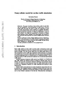
Figure 1: The main window of the TSF system
very easy to adopt the system to any other real road network. The system was developed in C# language using .NET technology and can be run on computers with installed .NET Framework (NET, 2009) in version 2.0 or higher (MS Windows XP/Vista/7) or Mono.NET (MONO, 2009) in version 2.0 or higher (Linux and Mac OS X). Maps and road network description come from the OpenStreetMap project (OSM, 2009). 3.1 Functionality of the TSF In this subsection we briefly present the most important features of the TSF system: • • • • • • •
Graphical user interface Simulation of vehicular traffic Generation of routes for drivers Editing settings of traffic lights Editing distribution of start points and destination points Specifying streets and areas which should be monitored during simulation Outputing data during simulation
3.1.1 Graphical User Interface One of the most characteristic features of the TSF system is a comprehensive graphical user interface (GUI). The main window of the application contains a city map which can be zoomed in, zoomed out and moved (Figure 1).
Traffic Simulation Framework
647
In addition, the user may specify elements displayed on a map. It is possible to display the following information: • • • • • • •
Locations and velocities of cars Locations and states of traffic lights All streets and all types of roads All vertices of the road network Average car velocities on every street Distribution of start and destination points Streets and regions which will be monitored during the simulation
3.1.2 Simulation of vehicular traffic The main functionality of the TSF system is to simulate a real vehicular traffic. A simulation process is based on the TSF model described in section 2.2. Currently system allows to simulate motion of about 106 cars in a real-time. This number is close to the real number of cars which participate in the real traffic in Warsaw (ZDM (2007)). Before start of the simulation, user may specify initial number of cars, time of a single step, number of cars which start driving after specified number of steps and some additional parameters related with driver’s behaviour (i.e. turningParameter and crossroadParameter which are used in the TSF model). 3.1.3 Generation of routes for drivers All vehicles which participate in the simulation have specified default routes. A single route is a sequence of vertices of the road network which is represented as directed graph G = (V, E). The first element of that sequence is always a start point and the last element is a destination point. The route is always a path in G between start point and destination point. The user is able to calculate any number of routes before start of the simulation. It is also possible to save calculated routes and read them later from a file. A single route is calculated as follows: Algorithm 2 The general algorithm for calculating routes Require: G = (V, E) - road network, S - start points distribution, D - destination points distribution Random v ∈ V with a distribution S Random w ∈ V with a distribution D route := the path in G between v and w return route The TSF assumes that drivers generally choose routes which are optimal in terms of time required to reach a destination point. Every edge in graph G represents some real-world street (or part of a street) which is characterized by a distance and type. Every type of roads has its own default maximal velocity
648
Pawel G´ ora
(which may be also modified by users), so it is possible to calculate a default time required to cover any street. Thanks to that, calculating routes means finding a shortest path betweeen 2 vertices in the graph and it could be calculated in many ways. In TSF we implemented A∗ algorithm with heuristic related with the real-world distance between vertices. 3.1.4 Editing settings of traffic lights Traffic signals are very important in the TSF model and have also great impact on the real traffic. The TSF input data contains information about location of traffic signals, but it is impossible to get the real-world signals synchronization. In the TSF all traffic lights are characterized with the following attributes: • • • •
period of green phase period of red phase initial phase number of steps to change a phase.
The TSF provides tools for adding, modifying and deleting traffic lights from the city map. All can be achieved just be clicking on a map and providing attributes, just like in figures 2 and 3.
Figure 2: An exemplary synchronization of traffic lights
Figure 3: A form to provide values for a traffic signal
3.1.5 Editing distribution of start points and destination points We have already described the process of calculating routes. We have mentioned that start and destination points are randomly generated from a given distribution. In the TSF this distribution is initiated with help of real-world data gathered from the automatic measurements (ZDM, 2007). However, it is also possible to edit those distributions manually from the graphical user interface. First, we have to describe how distributions are represented.
649
Traffic Simulation Framework
The whole city map is divided into square regions, each of them represents the real 500m×500m square. Every region has attributes rankstart and rankdestination which may take values from a set {0, 1, 2, 3, 4}. Every vertex of the city road network has also the same attributes and values of those attributes are the same as values of a region in which the vertex is located. The rankstart parameter implicates a probability of being selected as a starting point, similarly the parameter rankdestination implicates the same in case of destination points. Let rankstart (v) be a value of rankstart attribute for the vertex v. Then: ∀v∈V P (v is selected as a starting point) = P
rankstart (s) w∈V rankstart (w)
The similar equation is in case of destination points. The TSF allows to display and modify values of attributes rankstart and rankdestination by marking chosen regions on a map. It is showed in Figure 4.
Figure 4: An exemplary distribution of start points
3.1.6 Specifying monitored streets and areas The TSF gives opportunity to select edges from a road network which will be monitored during the simulation. Then, in every step some data from that edges will be collected and possibly printed out to a file. It is possible to select any single edge in the graph, by marking its vertices on a map. The user may also select all edges from bigger area by marking appropriate
650
Pawel G´ ora
rectangle on a map. The simulator’s GUI allows to modify selected areas, give them names, display on a map or delete from the set of monitored regions. Figure 5 shows an exemplary monitored regions defined by a user and Figure 6 presents the corresponding set of edges.
Figure 5: An exemplary set of monitored regions
Figure 6: An exemplary set of monitored edges
3.1.7 Outputting simulation data The main goal of monitoring parts of road network is to collect data from the simulated traffic. All data are being saved into files and can be later processed by external tools.
Traffic Simulation Framework
651
The application outputs information about “static” elements of the road network (graph description, initial traffic lights synchronization) as well as information about motion of all cars within monitored regions. In every simulation step and for every car from selected areas program writes to file the following information: • • • • • •
T ime - current step CarID - id of the car EdgeID - id of an edge (road) on which the car is located LaneID - id of a lane of edge EdgeID on which the car is located Location - distance between car and the beginning of edge EdgeID V elocity - current car velocity.
4 Applications of the TSF The main application of the Traffic Simulation Framework is simulating and investigating the real vehicular traffic in big agglomerations. It can be used to support efforts of scientists who try to understand vehicular traffic and engineers who work on designing and organizing road traffic in cities. The system may help in identifying roads with poor capacity and regions which are especially exposed to appearence of traffic jams. In the future it may also serve as a tool for predicting evolution of traffic. Currently, TSF is especially a great source of data that can be used to test various concepts and techniques of machine learning, data mining, process mining and related fields. Program produces data which illustrate complex phenomenon of vehicular traffic. Data come from sequential steps and concern motion of many agents over time. Agents are independent, but they constantly interact and influence on each other which make vehicular traffic difficult to describe. System will be used to test methods of discovering models of complex processes from data, based on domain knowledge represented by concept ontology. Data will serve to build hierarchical classifiers for identifying patterns e.g., relevant to forming traffic jams. Those algorithms may be then implemented in the TSF and help in automated planning of traffic, i.e. synchronization of traffic signals. If successful, it may be a very important progress in planning and organizing vehicular traffic in cities. Finally, TSF will be also adopt to test and compare various evolutionary algorithms (first of all: genetic algorithms) for finding optimal setting traffic ligths. The problem is proved to be NP-hard (Yang, 1996), so any good results in the field may be extremely valuable. Previous works report that applying evolutionary algotihms may bring some interesting results (Chen, 2007).
5 Possible extentions Despite the fact that TSF is still in a development phase, it already possesses wide functionality, which make it a convenient and useful tool for simulating and
652
Pawel G´ ora
investigating a phenomenon of road traffic. The system is planned to be expanded in the following directions: • Enabling parallel computing using NVidia CUDA architecture and CUDA.NET environment. It may result in much greater computational power and faster simulations. • Creating a programming environment in which users will be able to implement their ideas of traffic simulating, traffic oganizing and signals synchronizing. • Supporting other map formats with better precision.
6 Conclusions In the paper we have presented the Traffic Simulation Framework, an information system for simulating vehicular traffic. We have briefly described a theoretical background and mathematical aspects which were involved in implementation of the TSF. In addition, the most important functionalities of the system were also mentioned and discussed. TSF may have a wide range of applications, especially as a tool for investigating and forecasting vehicular traffic in cities, but also as a source of data which can be applied to test various algorithms and concepts related with machine learning, data mining, parallel computing, intelligent control systems and evolutionary distributed systems. Despite extended functionalities, there are still many ways to research, develop and improve the system in the future in order to apply this tool in real-life projects. Acknowledgements The research has been partially supported by the grant N N516 368334 from Ministry of Science and Higher Education of the Republic of Poland.
References Andreas Schadschneider (2000), Statistical Physics of Traffic Flow, Physica A285, 101. Andreas Schadschneider (1999), The Nagel-Schreckenberg model revisited, The European Physical Journal B, Volume 10, Issue 3, pp. 573-582. Oliver Biham, A. Middleton, D. Levine, (1992), The Self organization and a dynamical transition in traffic flow models, Physical Review A 46 R6124. Kai Nagel, Michael Schreckenberg, (1992), A cellular automaton model for freeway traffic, Journal de Physique 2 (1992), pp. 2221-2229. D. Chowdhury, A. Schadschneider, Self-organization of traffic jams in cities: effects of stochastic dynamics and signal periods, (1999), Physical Review E (Statistical Physics, Plasmas, Fluids, and Related Interdisciplinary Topics), Volume 59, Issue 2. OpenStreetMap Project, an official website: http://www.openstreetmap.org. Microsoft .NET Framework, an official Microsoft .NET Framework website: http://www.microsoft.com/NET/. Mono.NET Project, an official website: http://www.go-mono.com.
Traffic Simulation Framework
653
Zarzad Drog Miejskich w Warszawie, Informacja o ruchu na drogach ukladu podstawowego m.st. Warszawy wg Automatycznych Pomiarow Ruchu -ZDM 2007, website: http://www.zdm.waw.pl/informacje/badania-i-analizy/informacja-o-ruchuna-drogach-ukladu-podstawowego-mst-warszawy.html C. B. Yang, Y. J. Yeh, The model and properties of the traffic light problem, Proc. of International Conference on Algorithms, Kaohsiung, Taiwan, pp. 19-26, Dec. 1996 Shiuan-Wen Chen, Chang-Biau Yang, Yung-Hsing Peng, Algorithms for the Traffic Light Setting Problem on the Graph Model, website: http://par.cse.nsysu.edu.tw/ cbyang/person/publish/c07traffic.pdf NVidia CUDA Project, an official NVidia CUDA website: http://www.nvidia.com/object/cuda home.html# CUDA.NET Project, an official CUDA.NET website: http://www.gass-ltd.co.il/en/products/cuda.net/