In video based surveillance applications, a basic and important approach called ... But it will totally fail when foreground ... can be found but in hidden form [7].
Traffic Video Segmentation Using Adaptive-K Gaussian Mixture Model Rui Tan, Hong Huo, Jin Qian, and Tao Fang Institute of Image Processing and Pattern Recognition, Shanghai Jiao Tong University, Shanghai 200240, China {tanrui, huohong, qianjinml, tfang}@sjtu.edu.cn
Abstract. Video segmentation is an important phase in video based traffic surveillance applications. The basic task of traffic video segmentation is to classify pixels in the current frame to road background or moving vehicles, and casting shadows should be taken into account if exists. In this paper, a modified online EM procedure is proposed to construct Adaptive-K Gaussian Mixture Model (AKGMM) in which the dimension of the parameter space at each pixel can adaptively reflects the complexity of pattern at the pixel. A heuristic background components selection rule is developed to make pixel classification decision based on the proposed model. Our approach is demonstrated to be more adaptive, accurate and robust than some existing similar pixel modeling approaches through experimental results.
1
Introduction
In video based surveillance applications, a basic and important approach called background subtraction is widely employed to segment moving objects in the camera’s field-of-view through the difference between a reference frame, often called background image, and the current frame [1]. The accuracy of the background image quite impacts on output quality of the whole system, but the task to retrieve an accurate background is usually overlooked in many video based surveillance systems. It is complicated to develop a background modeling procedure that keeps robust in changeful environment and for longtime span. The simplest background reconstruction scheme adopts the average of all historical frames as the background image, which contains both real background component and foreground component. Consequently, the arithmetic average method causes confusion. As an improved version, Running Gaussian Average [1] is employed instead of arithmetic average, for each pixel (x, y), current background value Bj (x, y) is given by Bj (x, y) = αI(x, y) + (1 − α)Bj−1 (x, y),
(1)
where I(x, y) is current intensity, Bj−1 (x, y) is last background value and α is a learning rate often chosen as trade-off between the stability of background and the adaptability for quick environmental changes. Confusion problem also can N. Zheng, X. Jiang, and X. Lan (Eds.): IWICPAS 2006, LNCS 4153, pp. 125–134, 2006. c Springer-Verlag Berlin Heidelberg 2006 �
126
R. Tan et al.
not be avoided in this approach. Autoscope system [2] adopts such approach but a background suppression procedure is needed to eliminate the confusion. Temporal Median Filter [1], a nonparametric, welcomed and applicable approach, uses temporal median value of recent intensities in a length-limited moving window as the background at each pixel. Temporal Median Filter can generate an accurate background image under the assumption that the probability of real background in sight is over 0.5 in initialization phase, and the computational load of Temporal Media Filter is predictable. But it will totally fail when foreground takes up more time than background. N. Friedman et al. [3] first use Gaussian Mixture Model (GMM) to model the pixel process. Their model contains only three Gaussian components corresponding to road background, moving vehicles and dynamic casting shadows. Meaning of their approach lies in pixel modeling and a wise EM framework to train GMM, but it is not clear if the real scene doesn’t fit such a three components pattern. C. Stauffer et al. [5], [6] work out a successful improvement based on N. Friedman et al.’s model. They model each pixel process as a GMM with K Gaussian components, where the constant K is from 3 to 5, and then employ a heuristic rule to estimate background image. In their approach, the number of components, K, is a pre-defined constant for each pixel. Reversible Jump Markov chain Monte Carlo (RJMCMC) methods can be used to construct GMM with an unknown number of components [10], but there is no realtime version of RJMCMC for video processing. In this paper, we try to present an engineering oriented and realtime approach to construct GMM with an unknown number of components through a modified EM procedure. As a result, complicated regions in the video is described by more components adaptively, and simple regions with fewer components vice versa. The rest of this paper is organized as follows: Section 2 briefly introduces GMM modeling using EM algorithm. AKGMM learned by a modified EM procedure and a heuristic background components selection rule are proposed in Section 3. In section 4, comparative experimental results are analyzed and section 5 concludes this paper.
2
Related Work
Parametric probabilistic approaches in image processing usually treat each pixel independently and try to construct a statistical model for each pixel [3], [4], [6]. GMM is such a prevalent model usually trained using an iterative procedure called Expectation Maximum algorithm (EM algorithm). EM algorithm is introduced briefly in this section. Considering the values of a particular pixel over time as a pixel process, its history becomes χ = {xj = Ij (x, y)}nj=1 ,
(2)
where Ij (x, y) is grayscale or color vector at time j for pixel (x, y). A mixture model of Gaussian distributions can be set up on χ at this pixel to gain on the underlying PDF [7],
Traffic Video Segmentation Using Adaptive-K Gaussian Mixture Model
127
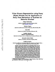
Fig. 1. A pixel process is constituted by values of a particular pixel over time. For each pixel in the frame, a statistical model is built upon the corresponding pixel process.
f (x|Θ) =
K �
ωi η(x|Θi ),
(3)
i=1
where ωi is the normalized weight of ith Gaussian component Ci , so η(x|Θi ) is PDF for Ci which can be replaced by
�K i=1
1 1 x − μi 2 η(x|Θi ) = √ exp[− ( ) ]. 2 σi 2πσi
ωi = 1;
(4)
Theoretically, the Maximum-Likelihood root of parameters Θ = {ωi , Θi }K i=1 can be found but in hidden form [7]. In practice, mixture models can be learned using EM [3], [8]. Because of the requirement of realtime system, an online EM version [3], [9] was proposed which converges to local expectation maximum point with high probability. In this variant of EM, three sufficient statistics, Ni , Si , Zi are considered, where Ni represents �the count of samples belonging to Ci ; Si is the sum of these samples, Si = xj ∈Ci xj ; Zi represents the sum of � the outer product of these samples, Zi = xj ∈Ci x2j /n. Consequently, the model parameters can be calculated from these sufficient statistics as follow, Ni ωi = �K k=1
Nk
,
μi =
Si , Ni
σi2 =
1 Zi − μ2i . Ni
(5)
When a new sample xj comes in, these sufficient statistics are updated as follow, Nij = Nij−1 + P (X ∈ Ci |X = xj , Θj−1 ), Sij = Sij−1 + xj P (X ∈ Ci |X = xj , Θj−1 ), Zij = Zij−1 + x2j P (X ∈ Ci |X = xj , Θj−1 ),
(6)
where P (X ∈ Ci |X = xj , Θ) =
ωi η(xj |Θi ) P (X ∈ Ci , X = xj |Θ) = , P (X = xj |Θ) f (xj |Θ)
(7)
and we choose {Ni0 , Si0 , Zi0 }K i=1 as initial values of these sufficient statistics. From j the updated {Nij , Sij , Zij }K i=1 , we can compute Θ . If the underlying PDF is
128
R. Tan et al.
stationary, Θj will converge to local expectation maximum point with high probability in long run [3], [9].
3
Adaptive-K Gaussian Mixture Model
R. Bowden et al. have successfully segmented low resolution targets using C. Stauffer et al.’s fixed K model [11], and they argue that it is not suitable for large scale targets segmentation [11]. The detailed information of large moving objects’ appearance, i.e., color, texture and etc, makes the pattern of pixels in the track of objects much complicated. In other words, the objects’ track regions hold a complex pattern mixed with background components and kinds of object appearance components, but other regions hold just a stable background pattern. And in practice, the difference among different regions, which is impacted by many factors, i.e., acquisition noise, light reflection, camera’s oscillation caused by wind, is also complicated. It is not suitable to describe every pixel in field-ofview using a mixture model with fixed K Gaussian components as C. Stauffer et al. did [5], [6]. We try to describe those pixels with complex pattern using more Gaussian components adaptively, in other words, bigger K at those pixels, and those simple pixels using fewer components vise versa. In such strategy, a more accurate description of the monitoring region is expected. In video based traffic surveillance applications, vehicles which are relatively large size targets are tracked. 3.1
Pixel Modeling
When the first video frame comes in, a new Gaussian component is created at each pixel with the current grayscale as its mean value, an initially high variance, and low prior weight. In the following, at each pixel, a new instance is used for updating the model using (6) if a match is found. A match is defined as a pixel value within 2.5 standard variance of a component. If no match is found, a new Gaussian component is created and no existing component is disposed. Then, two problems arise: those three sufficient statistics, {Ni , Si , Zi }, increase unlimitedly while more frames are captured; K may also increase unlimitedly at � a particular pixel, so the computational load will increase drastically. Firstly, K j−1 < L, {Ni , Si , Zi } are updated using (6); otherwise we define a if i=1 Ni forgetting rate as follow, �K Nij−1 β = �K i=1 j−1 , +1 i=1 Ni
(8)
then those sufficient statistics are updated using Nij = β[Nij−1 + P (X ∈ Ci |X = xj , Θj−1 )], Sij = β[Sij−1 + xj P (X ∈ Ci |X = xj , Θj−1 )], Zij = β[Zij−1 + x2j P (X ∈ Ci |X = xj , Θj−1 )].
(9)
Traffic Video Segmentation Using Adaptive-K Gaussian Mixture Model
129
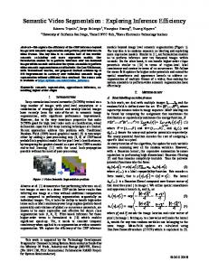
� As a result, K i=1 Ni will be a constant near by L which is an equivalent time constant. Secondly, every L frames, each Gaussian component is checked at any pixel whether coefficient of some component Ck , that is ωk , is below a pre-defined threshold ωT . If inequality ωk < ωT holds, component Ck is discarded because the inequality means there are too few evidences to support that component which is inspired by low-probability events. 1/L is a reasonable value for ωT , because a component supported by less than one evidence in L frames shouldn’t be maintained. After a number of frames are processed, K will adaptively reflects the complexity of pattern at each pixel, in other words, we can set up a more accurate description of the monitoring region. In this case, computational cost is mainly allocated for complicated regions, such as tracks of the moving objects. Figure 2(b) shows a K-image formed by the components’ number at each pixel, where grayscale encodes K accumulated by 200 frames using AKGMM. As our expectation, pixels in the three lanes have more Gaussian components than pixels in other areas, i.e., barriers by the road.
(a)
(b)
(c)
(d)
Fig. 2. (a) Monitoring scene on a highway; (b) shows a image formed by the components’ number where grayscale encodes K; (c) is the background image formed by mean value of the first Gaussian component at each pixel; (d) plots PDF at point A labeled in (a)
3.2
Background Estimation
For GMM, measurement ω/σ is proposed to be positively related to the probability of being background component [5], [6]. Heuristically, C. Stauffer et al. select the first B components in the sequence of all components ordered by ω/σ as background, where b � B = arg min( ωi > T ). b
(10)
i=1
In such strategy, T is a threshold related to occupancy in traffic applications. Such background estimation may fail in some cases, i.e., large flow volume, traffic jam, if the background is just judged from occupancy. A searching procedure is developed to estimate background in our framework. Assume the first component in the sequence of components ordered by ω/σ must be a part of background, and background components set B includes only the
130
R. Tan et al.
first component initially while the other components are labeled non-background. In the iterative searching phase, a non-background component Cnb is labeled background and included into B if μnb ∈ [μb − 3σb , μb + 3σb ],
∃Cb ∈ B,
(11)
where μnb is mean value of Cnb ; Cb is some background component with mean value μb and standard variance σb . The iteration ends until no such component Cnb can be found. If a background image is needed, we choose the mean value of the first component of B, in which elements are also ordered by ω/σ, at any pixel to form the background image. Figure 2(c) shows such a background image accumulated by the first 100 frames. Figure 2(d) plots PDF at point A labeled in Fig.2(a), in which five components are included. Solid line represents two background components selected by our searching procedure, and dotted line represents the other three non-background components. Our experimental results will show that our simple iterative procedure generates accurate background model in many traffic cases. 3.3
Foreground Segmentation
In terms of the background components set B updated in the previous searching procedure, a new grayscale at pixel (x, y) is identified as moving vehicle if the current grayscale matches no component in B when dynamic casting shadow is out of consideration. If vehicles cast moving shadows, non-background pixels should be segmented into vehicles and their casting shadows, otherwise the foreground segmentation will be enlarged wrongly. Many shadow detection algorithms are proposed, but most of them are too complex. In our framework, we adopt a simple shadow detection algorithm called Normalized Cross-Correlation algorithm (NCC algorithm) proposed by Julio et al. [12] to refine the segmentation if dynamic casting shadow exists. NCC explores the relationship between casting shadow and background, that is, the intensity of shadowed pixel is linear to the corresponding background, so the background image provided by AKGMM is used to detect shadows. An example of the segmentation refinement applied to the original frame with shadow is depicted in Fig.3(b). In this figure, white areas correspond to moving vehicles and gray areas correspond to shadow detection. Figure 3(c) shows the final foreground segmentation result after applying morphological operators to eliminate gaps and isolated pixels.
4
Experimental Results
Following comparative experiments demonstrate the performance of our proposed algorithm on two groups of traffic image sequences. Dataset A is recorded
Traffic Video Segmentation Using Adaptive-K Gaussian Mixture Model
(a)
(b)
131
(c)
Fig. 3. Segmentation result using AKGMM and NCC. (a) is the original frame; (b) shows the segmentation (shadowed pixels are represented by light gray); (c) is morphological post-processing result after shadow removal.
on a highway; dataset B is by an intersection on a ground road, and the camera oscillates drastically in the wind. The video size is 320x240 and shadow detection is incorporated in following experiments. In order to distinguish our framework from C. Stauffer et al.’s, we name their model Fixed-K Gaussian Mixture Model (FKGMM) in the following. 4.1
Reflection
In this experiment, FKGMM maintains 3 components at each pixel, while the average of components’ number in AKGMM is about 6. In the Fig.4(d), we can see there are more false alarm pixels in the output of FKGMM, and our shadow areas have better texture than theirs. Whenever a large vehicle passes by the camera, reflection from the large vehicle impacts on the quantification of the camera in the whole field-of-view. Column 2 and 3 show the difference between the two models in such case. In FKGMM, a meaningful component may be substituted by a new one which is inspired by the sudden reflection to keep K as a constant. Consequently, the sudden reflection is classified as dynamic casting shadow. In contrast, AKGMM gives a more accurate background description, and no component will be destroyed by the sudden reflection, so AKGMM works better in such cases. 4.2
Camera’s Oscillation
In outdoor applications, camera’s oscillation caused by wind should be taken into consideration. In this robustness experiment in case of camera’s oscillation, 5 components are maintained and the threshold T in (10) is set to 0.5 for FKGMM. The background selected by FKGMM will be unimodal at most pixels. As a result, edges of the ground marks and static objects by the road are identified as non-background because of the oscillation. By increasing T , FKGMM will behave better because the background becomes multimodal, but the confusion problem will occur as analyzed in next subsection. The K-image of AKGMM depicted in Fig.5(d) illuminates that these edges are described more accurately. After an opening then a closing morphological operation, our framework takes on better robustness than C. Stauffer et al.’s.
132
R. Tan et al.
(a)
(b)
(c)
(d)
(e)
(f)
(g)
(h)
(i)
Fig. 4. Corresponding segmentations on dataset A. Top row: the original images at frames 1443, 2838, 2958. Middle row: the corresponding segmentation using C. Stauffer et al.’s model (shadowed pixels are represented by light gray). Bottom row: the segmentation using AKGMM.
(a)
(b)
(c)
(d)
(e)
(f)
Fig. 5. Segmentation on dataset B in case of camera’s oscillation. (a): the original image at frame 422; (b)-(c): segmentation using FKGMM and corresponding morphological post-processing result; (d): K-image of AKGMM; (e)-(f): segmentation using AKGMM and corresponding morphological post-processing result.
Traffic Video Segmentation Using Adaptive-K Gaussian Mixture Model
4.3
133
Stationary Vehicles
In front of intersections, vehicles occasionally stop to wait for pass signal. To detect stationary vehicles is a typical problem in video based traffic surveillance. In dataset B, the vehicles stop for about 15 seconds, 375 frames equivalently, every 45 seconds’ pass. Figure 6(a) and Fig.6(d) represent such a move-to-stop process for about 4 seconds. The threshold T is adjusted to 0.9 to keep FKGMM robust in oscillation. The Gaussian components which correspond to the stationary vehicles grow so quickly that these components are included into background according to (10). Consequently, the stationary vehicles incorporate into background as showed in Fig.6(e). In our framework, the incorporation occurs provided that the stationary vehicles cover those pixels more frames than the time constant L. By choosing an appropriate L, our system keeps robust both in camera’s oscillation and stationary vehicles case.
(a)
(b)
(c)
(d)
(e)
(f)
Fig. 6. Segmentation on dataset B in case of stationary vehicles. (a): original image at frame 1680; (b)-(c): segmentation of (a) using FKGMM and AKGMM; (d) original image at frame 1768; (e)-(f): segmentation of (d) using FKGMM and AKGMM.
5
Conclusions and Future Work
A visual traffic surveillance application oriented, probabilistic approach based large scale moving objects segmentation strategy is presented in this paper. In our strategy, a modified online EM procedure is used to construct Adaptive-K Gaussian Mixture Model at each pixel, and a heuristic background components selection rule is developed to generate accurate background and make pixel classification decision. Our approach shows good performance in terms of adaptability, accuracy and robustness, but the computational load is unpredictable because of the very adaptability. We can constrain the computational load by applying our approach just in small Region of Interest (ROI). Reasonable heuristic background estimation rules and adaptability for kinds of environmental changes
134
R. Tan et al.
need more study. Some intro-frame tasks, such as vehicle tracking, can be studied based on the object segmentation. Acknowledgements. This research is supported in part by Demonstrative Research of WSN Application in Transportation Systems administered by Shanghai Science and Technology Committee under grant 05dz15004.
References 1. M. Piccardi, “Background Subtraction Techniques: A Review,” in 2004 IEEE International Conference on Systems, Man and Cybernetics, pp.3099-3104. 2. P. G. Michalopoulos, “Vehicle Detection Video Through Image Processing: The Autosope System,” IEEE Trans. on Vehicular Technology, vol.40, No.1, February 1991. 3. N. Friedman and S. Russell, “Image Segmentation in Video Sequences: A Probabilistic Approach,” in Proceedings of the 13th Conference on Uncertainty in Artificial Intelligence(UAI), San Francisco, 1997. 4. C. R. Wren, A. Azarbayejani, T. Darrell, and A. P. Pentland, “Pfinder: Real-time Tracking of the Human Body,” IEEE Trans. on Pattern Analysis and Machine Intelligence, vol.19, No.7, July 1997. 5. C. Stauffer and W.E.L. Grimson, “Adaptive Background Mixture Models for ReadTime Tracking,” in Proceedings of the IEEE Computer Society Conference on Computer Vision and Pattern Recognition, vol.2, pp.246-252, 1999. 6. C. Stauffer and W.E.L Grimson, “Learning Patterns of Activity Using Real-Time Tracking,” IEEE Trans. on Pattern Analysis and Machine Intelligence, vol.22, No.8, August 2000. 7. Z. R. Yang and M. Zwolinski, “Mutual Information Theory for Adaptive Mixture Models,” IEEE Trans. on Pattern Analysis and Machine Intelligence, vol.23, No.4, April 2001. 8. A. Dempster, N. Laird, and D. Rubin, “Maximum Likelihood From Incomplete Data via the EM Algorithm,” Journal of the Royal Statistical Society, 39(Series B):1-38, 1977. 9. R. M. Neal and G. E. Hinton, “A View of the EM Algorithm That Justifies Incremental, Sparse, and Other Variants,” Learning in Graphical Models, pp.355-368, 1998. 10. S. Richardson and P.J. Green, “On Bayesian Analysis of Mixtures with an Unknown Number of Components,“ Journal of the Royal Statistical Society, 60(Series B):731-792, 1997. 11. P. KaewTraKulPong and R. Bowden, “An Adaptive Visual System for Tracking Low Resolution Colour Targets,” in Proceedings of British Machine Vision Conference 2001, vol.1, pp.243-252, Manchester UK, September 2001. 12. Julio Cezar Silveira Jacques Jr, C. R. Jung, and S. R. Musse, “Background Subtraction and Shadow Detection in Grayscale Video Sequences,” in Proceedings of SIBGRAPI 2005-Natal-RN-Brazil, 2005.