Trailing Mobile Sinks: A Proactive Data Reporting Protocol for Wireless Sensor Networks Xinxin Liu, Han Zhao, Xin Yang Computer & Information Science & Eng. University of Florida Email:{xinxin,han,xin}@cise.ufl.edu
Xiaolin Li Electrical and Computer Eng. University of Florida Email:
[email protected]
Abstract—In Wireless Sensor Networks (WSN), data gathering using mobile sinks typically incurs constant propagation of sink location indication messages to guide the direction of data reporting. Such behavior is undesirable, especially when the sensor network scale increases, as frequent message flooding will cause serious congestion in network communication and significantly impair the sensor network lifetime. In this paper, we propose a proactive data reporting protocol, SinkTrail, which achieves energy efficient data forwarding to multiple mobile sinks, and effectively reduces the number of sink location broadcasting messages. SinkTrail is unique in two aspects: (1) it allows sufficient flexibility in the movement of mobile sinks to dynamically adapt to unknown terrestrial changes; and (2) without assistance of GPS or predefined landmarks, SinkTrail establishes a logical coordinate system for predicting and tracking mobile sinks’ locations, thereby significantly saves energy consumed during the data reporting process. We systematically analyze the impact of several design factors in SinkTrail and explore potential design improvements. The simulation results demonstrate that SinkTrail outperforms the Frequent Flooding Method (FFM) in finding shorter routing path and consumes less energy during data gathering process.
Ning Wang Biosystems and Agriculture Eng. Oklahoma State University Email:
[email protected]
Fig. 1. A photograph showing a typical farmland of irregular shapes. A mobile sink’s movement in such environment is constrained.
I. I NTRODUCTION Wireless sensor networks (WSNs) are envisioned to consist of thousands of low-cost sensor nodes that are capable of gathering information from their immediate vicinity, processing sensed data, and communicating with each other via short-range radio links. A majority of WSN applications are concerning environmental information collection, e.g., habitat monitoring [13], and precision agriculture [10]. In these applications, sensor nodes are deployed in wild areas with few human interventions. Since sensor nodes have limited battery life, energy saving is of paramount importance in the design of sensor network protocols. Recent research on data collection reveals that, rather than reporting data through long, multihop, and error-prone routes to a static sink using tree or cluster network structure, allowing and leveraging sink mobility is more promising for energy efficient data gathering [1]. Mobile sinks, such as animals or vehicles equipped with radio devices, are sent into a field and communicate directly with sensor nodes. As such data transmission path is greatly shortened and energy consumption for relaying is reduced. However, data gathering using mobile sinks introduces new challenges to sensor network applications. As sink location changes constantly, routing algorithms designed for static sink The work presented in this paper is supported in part by National Science Foundation (grants CNS-0709329 and CNS-0923238) and OCAST.
Fig. 2. Comparison of routing methods: FFM vs. SinkTrail. A mobile sink moves from trail point 1 to trail point 2 in a sensor network deployed in a wild area. Black solid route represents data report message path in FFM (without location prediction), it takes 6 hops to trail point 2. Whereas red dashed route represents predictive SinkTrail routing, taking only 4 hops to the mobile sink’s current location.
are no longer suitable. For a WSN that consists thousands of sensors, gathering data by querying each sensor node individually will incur significant delay, thus is not feasible for many applications. Although several mobile elements scheduling (MES) protocols have been proposed to achieve efficient data collection via controlled sink mobility [12], [19], [24], determining a perfect moving trajectory for a mobile sink is itself an NP-hard problem [12], and may not be able to adapt to constrained access areas and changing field situations. One example is precision agriculture applications, e.g. Fig. 1, where mobile sinks collecting data most likely follow trails or field boundaries in order to not damage crops, and change trajectories dynamically according to farmland situations.
Data dissemination protocols, such as Directed Diffusion [8] and DRP [2], suggest that a mobile sink announce its location information frequently throughout the network. We refer to this class of methods as Frequent Flooding Method (FFM). An example data reporting path of FFM is presented using black solid route shown in Fig. 2. FFM consumes large amount of energy on broadcasting, and wastes extra energy to detour large data packets (originally target at previous sink location, now change to current sink location). To improve the scalability and energy efficiency in FFM, we require data to be transmitted via the shortest route to the mobile sink’s future locations, as observed in the red dashed route in Fig. 2. Therefore if sensors can predict the mobile sink’s movement, the energy consumption would be greatly reduced and data packets handoff would be smoother. In this paper we propose SinkTrail, a proactive, greedy data forwarding protocol that is self-adaptive to various application scenarios. In SinkTrail, mobile sinks move continuously in the field in relatively low speed, and gather data on the fly. Control messages are broadcasted at certain points in much lower frequency than FFM. These positions are viewed as “footprints” of a mobile sink. Viewing each footprint as a virtual landmark, it is easy for a sensor node to identify its hop count distances to these landmarks. These hop count distances combined represent the sensor node’s coordinate in the logical coordinate space. Similarly, coordinate of the mobile sink is its hop count distances from the current location to previous virtual landmarks. Having the destination coordinate and its own coordinate, each sensor node greedily selects next hop with the shortest logical distance to the mobile sink. As a result SinkTrail solves the problem of movement prediction for data gathering with mobile sinks. Our contributions for proposing SinkTrail are three-fold: first, we propose a unique logical coordinate representation for tracking mobile sinks without assistance of GPS devices or predefined landmarks. Second, we design a novel lowcomplexity dynamic routing protocol for data gathering with one or multiple mobile sink(s), which effectively reduces average route length and lower total energy consumption. Third, the impacts of several design parameters of SinkTrail are explored, and improvements to the original SinkTrail protocol are also suggested to guide the deployment in realworld applications. The rest of this paper is organized as follows. Section II presents related work. The protocol design is introduced in Section III. Performance of SinkTrail is analyzed and investigated in Section IV. Section V proposes design improvements to SinkTrail, and Section VI concludes with a summary of our work. II. R ELATED WORK Due to its energy efficient property, leveraging mobile sinks in sensor data collection becomes popular in the past few years. In this section we review related research of this topic. At the first look, multicasting is the most natural solution to track the moving mobile sink. In [7], a spatial-temporal
multicast protocol is proposed to establish a delivery zone ahead of mobile sink’s arrival. Control messages are flooded to wake up nodes in the delivery zone. Similarly, Park et al. [15] proposed DRMOS that divides sensors into “wake-up” zones to save energy. Fodor et al. [5] lowered communication overhead by proposing a restricted flooding method; routes are updated only when topology changes. Lou et al. [11] proposed that a mobile sink should move following a circle trail in deployed sensor field to maximize data gathering efficiency. One big problem of the multicasting methods lies in its flooding nature. Moreover, these papers either assumes mobile sinks move at fixed velocity and fixed direction, or move following a fixed pattern, which largely confine their application. The SinkTrail protocol with message suppression minimizes the flooding effect of control messages without confining mobile sink’s moving, thus is more attractive in real-world deployment. Another solution utilizes opportunistic data reporting. For instance in [17] the authors studied data collection performance when a mobile sink presents at random places in the network. The method relies heavily on network topology and density, and suffers scalability issues when all data packets are forwarded repeatedly in the network. Another category of methods, called mobile element scheduling (MES) algorithms [3], [12], [19]–[21], [24], considered controlled mobile sink mobility and advanced planning of mobile sink’s moving path. Ma et al. [12] focused on minimizing the length of each data gathering tour by intentionally controlling the mobile sink’s movement to query every sensor node in the network. When data sampling rates in the network are heterogeneous, scheduling mobile sinks to visit hot-spots of the sensor network becomes helpful. Example algorithms can be found in [3], [20], [21]. Although the MES methods effectively reduce the data transmission cost, they require a mobile sink to cover every node in the sensor field, which makes it hard to accommodate to large-scale, and introduces high latency in data gathering. Even worse, finding an optimal data gathering tour in general is itself an NP-hard problem [12], and constrained access areas or obstacles in the deployed field pose more complexity. Unlike MES algorithms, SinkTrail, with almost no constraint on the moving trajectory of mobile sinks, achieves much more flexibility to adapt to dynamically changing field situations while still maintains low communication overhead. SinkTrail uses sink location prediction and selects data reporting routes in a greedy manner. Previous research proposed location prediction and proactive data reporting can be found in [9] and [22] respectively. In [9] the authors used sequential Monte Carlo theory to predict sink locations. The TTDD protocol suggested in [22], constructed a two-tier data dissemination structure to enable fast data forwarding. It allowed nodes that are data sources proactively report data to the mobile sink. SinkTrail differs from these two papers in that it employs a different prediction technique that has lower complexity, and does not rely on the assumption of locationaware sensor nodes, which could be impractical for some real-world applications. The routing protocol of SinkTrail is
Algorithm 1 Mobile sink’s moving strategy /* Initialization */
2: msg.seqN ← 0;
msg.hopC ← 0; 4: Announces step size parameter K
/* Moving strategies */
6: while Not get enough data or Not timeout do
Move to next trail point ; msg.seqN← msg.seqN +1; Stop for a very short time to broadcast trail message ; 10: Concurrently listen for data report packets ; end while 12: End data gathering process and exit ; 8:
Fig. 3. Data gathering with one mobile sink: yellow stars indicate the mobile sink’s trail points, and sensor nodes maintain trail references as logical coordinates. Shaded areas stand for obstacles.
inspired by recent research on virtual coordinate routing [6], [14], [16]. Rao et al. [16] proposed a greedy algorithm for data reporting using logical coordinates rather than geographic coordinates. Fonseca et al. [6] presented vector form virtual coordinates, in which each element in the vector represented the hop count to a landmark node. SinkTrail adopts this vector representation, and uses past locations of the mobile sink as virtual landmarks. To the best of our knowledge, we are the first to associate mobile sink’s “footprint” left at moving path with routing algorithm construction. The vector form coordinates, called trail references, are used to guide data reporting without knowledge of the physical locations and velocity of the mobile sink. III. S INK T RAIL PROTOCOL DESIGN A. Problem formulation We consider a large scale, uniformly distributed sensor network N deployed in an outdoor area of irregular shape shown in Fig. 3. Nodes in the network communicate with each other via radio links. We assume the whole sensor network is connected, which is achieved by deploying sensors densely. We also assume sensor nodes are awake when data gathering process starts (by synchronization or a short “wake up” message). In order to gather data from N, we periodically send out some mobile sinks into the field. These mobile sinks are assumed to have sufficient power and equipped with radios and processors. A data gathering process starts from the time mobile sinks enter the field and terminates when: (1) enough data are collected (measured by a user defined threshold); and (2) there are no more data reports in a certain period. The SinkTrail protocol is proposed for sensor nodes to proactively report their data back to one of the mobile sinks. To illustrate our data gathering algorithm clearly, we first consider the scenario where there is only one mobile sink in N. The multiple mobile sinks scenario is discussed later. B. SinkTrail protocol with one mobile sink During the data gathering process, the mobile sink moves around in N with relatively low speed, and keeps listening for data report packets. It stops at some place for a very short time, broadcasts a message to the whole network, and moves on to
another place. We call these places “Trail Points”, and these messages “Trail Messages”. Example trail points are shown in Fig. 3. Let γ be the average transmission range, which is also one hop distance of radio transmission. Apparently two adjacent trail points should be separated by a distance longer than γ. To facilitate mobile sink tracking, we restrict that the distances between any two trail points are the same, denoted as Kγ, K ≥ 1. However, distribution of these trail points doesn’t necessarily follow any pattern. A trail message is a very short radio message sent by a mobile sink, it contains a sequence number (msg.seqN) and a hop count (msg.hopC) to the sink. The time interval between a mobile sink stops at one trail point and arrives at the next trail point is called one “move”. There are multiple moves during a data gathering round. The moving strategy of a mobile sink is summarized in Algorithm 1. In the SinkTrail algorithm, we use vectors called “Trail References” to represent logical coordinates in a network. The trail reference maintained by each node is used as a location indicator for greedy packet forwarding. All trail references are of the same size. We use the following notations throughout the protocol description. • • • • • • • • •
• •
ni : sensor node i N : total number of sensor nodes in N S: mobile sink M : number of mobile sinks vi : trail reference of node i ei j : the jth element in vi dv : trail reference size, dv = ||v|| b: average number of neighbors of each node λ: the most recent message sequence number a node has recorded πi : the ith trail point of S K: step size parameter for one move (a step of K hop counts is Kγ)
A sensor node has three functional states in the SinkTrail algorithm: “Prepare”, “Ready”, and “Post”. Fig. 4 displays the state transition of the sensor node. This state transition procedure consists mainly two phases. The first phase, called logical coordinate space construction, starts when the first trail message is received, and terminates before a node enters “Ready” state. During this phase, nodes update trail references corresponding to the mobile sink’s trail messages. After a node
Fig. 4.
State transition diagram for a sensor node.
leaves the “Ready” state, it enters the greedy forwarding phase, where nodes decide how to report data packets to the mobile sink. Algorithm 2 Trail reference update algorithm 2: 4: 6: 8: 10: 12: 14: 16: 18: 20: 22: 24:
while Data gathering process is not over do /* Receive a trail message */ if msg.seqN > λ then λ ← msg.seqN; Shift vi to left by one position ; ei dv ← msg.hopC + 1; msg.hopC ← msg.hopC +1; Rebroadcast message ; else if msg.seqN = λ then Compare ei dv with (msg.hopC + 1); if ei dv > (msg.hopC + 1) then ei dv ← msg.hopC + 1; msg.hopC ← msg.hopC +1; Rebroadcast message ; else Discard the message ; end if else if msg.seqN < λ then Discard the message ; end if end while /* Reset Variables */ For j = 1, . . . , dv ei j ← −1; λ ← −1;
1) Logical coordinate space construction: At beginning, all the trail references are initialized to [−1, −1, . . . , −1] of size dv . After the mobile sink S enters the field, it moves to its first trail point π1 , and broadcasts a trail message to all the sensor nodes in N. The trail message––is set to < 1, 0 >, indicating that this is the first trail message from trail point one, and the hop count to S is zero. The nodes nearest to S will be the first ones to hear this message. To check the “freshness” of a message, a node ni needs to compare the sequence number carried in this trail message with its λ, which represents the latest sequence numbers ni has seen. And λ is reset to −1 after each data gathering process finishes. If this is a new message, the λ variable will be updated by the new sequence number. And node ni ’s trail reference vi is updated as follows. First, every
Fig. 5. Example execution snapshot of SinkTrail: yellow stars indicate trail points, and directed arrows stand for the moving path of mobile sink.
element in vi is shifted to left by one position. Then, the hop count in the received trail message is increased by one, and replaces the right-most element ei dv in vi . After ni updates its trail reference, this trail message is rebroadcasted with the same sequence number and an incremented hop count. The same procedure repeats at all the other nodes in N. Within one move of S, all nodes in the network have updated their trail references according to their hop count distances to S’s trail point π1 . If a node receives a trail message with a sequence number equals to λ, but has a smaller hop count than it has already recorded, then the last hop count field in its trail reference is updated, and this trail message is rebroadcasted with the same sequence number and an incremented hop count. Trail messages that has sequence number less than λ will be discarded to eliminate flooding messages in the network. The steps described in Algorithm 2 summarizes the operations to update a trail reference. During the data gathering procedure, a node’s trail reference needs to be updated every time a new trail message is received. After each node in the network received dv distinct trail messages, the logical coordinate space is established. A snapshot of a part of the network N is shown in Fig. 5. Trail references, such as [3, 1, 3] or [4, 2, 2], are considered logical coordinates of the sensor nodes in a network. 2) Destination identification: The procedure of the SinkTrail algorithm described here is a flexible and straightforward way of logical coordinate space construction. Rather than scheduling a mobile sink’s movement, it allows a mobile sink to spontaneously stop at convenient locations according to current field situations. These sojourn places of a mobile sink, named trail points in SinkTrail algorithm, are footprints left by a mobile sink, and provide valuable information for tracing the current location of a mobile sink. Viewing these footprints as virtual sinks or landmarks, hop count information reflects the moving trajectory of a mobile sink. A logical, dv -dimensional coordinate space is then established. One advantage of SinkTrail is that the logical coordinate of a mobile sink keeps invariant at each trail point, given the continuous update of trail references. This is because the mobile sink’s hop count distance to its previous dv − 1
footprints are always K(dv − 1), K(dv − 2), . . . , K, and 0 to its current location. Therefore the logical coordinate [K(dv − 1), K(dv − 2), . . . , 0] represents the current logical location of the mobile sink. We call this coordinate “Destination Reference”. This destination reference does not necessary require a mobile sink to have linear moving trajectory. Although arbitrary movement of a mobile sink may deteriorate the accuracy of destination reference, it can still serve as a guideline for data reporting. Here we set K = 1 and dv = 3 to ease our presentation. A large value of K means even less broadcast frequency. (The impacts of mobile sinks’ moving pattern and broadcast frequency are investigated in section IV). Refer to Fig. 5, assume S is at trail point 3 now, then its destination reference should be [2, 1, 0]. When S moves to trail point 4, the coordinate space is updated based on trail points 2, 3, and 4, and destination reference of the mobile sink is still [2, 1, 0]. Algorithm 3 Greedy data forwarding algorithm /* Start a timer */ 2: if All elements of the trail reference are updated then 4: 6: 8: 10: 12: 14:
Start timer Ti = T0 − µ × ei dv Exchange trail references with neighbors end if /* When timer expires */ Set destination as [(dv − 1), . . . , 2, 1, 0] /* Probe mobile sink */ if A mobile sink is within radio range then Send data to the mobile sink directly else Choose the neighbor closest to destination as the next hop Forward all data to next hop end if
Fig. 6. Example execution snapshot of SinkTrail of multiple mobile sinks scenario.
whenever the mobile sink arrives at a new trail point. Although trail references may not be global identifiers, since route selection is conducted locally, they are good enough for the SinkTrail protocol. Because each trail reference has only 3 numbers, the size of exchange message is small. When a node has received all its neighbors’ trail references, it calculates their distances to the destination reference, [2, 1, 0], according to 2-norm vector calculation, and greedily choose the node with the smallest distance as next hop to relay data. If there is a tie we randomly choose one. The complete procedure of greedy forwarding is presented in Algorithm 3. Take the network in Fig. 5 as an example, when node n5 decides to report its data, it compares n3 and n4 ’s vector distance √ with [2, 1, 0]. Since n3 ’s distance to [2, 1, 0] is 11, and n4 ’s distance is 3, n4 is chosen as the next hop of n5 . C. SinkTrail protocol with multiple mobile sinks
3) Greedy forwarding: Once a node has updated the 3 elements in its trail reference (we use dv = 3 for easy understanding and clear presentation), it transfers from “Prepare” state to “Ready” state, and starts a timer that is inverse proportional to the right-most element in its trail reference. For example, in Fig. 5, node n5 ’s trail reference is [4, 2, 3], then the duration of its timer is set to T5 = T0 − µ × 3. Here, T0 and µ are predefined constants. The choice of timer function, T0 , and µ may vary. However, we assume the timer durations are significantly longer than the propagation time of a trail message, so that timers on all nodes are viewed as starting at the same time. This timer mechanism is mainly used to differentiate data reporting orders, so the clock on each sensor node doesn’t need to be perfectly synchronized. Since the right-most element in a node’s trail reference is the latest hop count information from this node to a mobile sink, the inverse proportional timers ensure that nodes faraway from S have shorter timer durations than those close to S, thus will start data reporting first. When a node’s timer expires, it goes into “Post” state, and initiates the data reporting process. Every sensor node in the network maintains a routing table of size O(b) consisting all neighbors’ trail references. This routing table is built up by exchanging trail references with neighbors, as described in Algorithm 3; and it is updated
The proposed SinkTrail protocol can be readily extended to multiple mobile sinks scenario with small modifications. When there are more than one sink in a network, each mobile sink broadcasts trail messages following Algorithm 1. Different from one sink scenario, a sender ID field, msg.sID, is added to each trail message to distinguish them from different senders. Algorithms executed on the sensor node side should be modified to accommodate multi-sink scenario as well. Instead of using only one trail reference, a sensor node maintains multiple trail references, each corresponds to a different mobile sink at the same time. Fig. 6 shows an example of two mobile sinks. Two trail references, colored in black and red, coexist in the same sensor node. In this way, multiple logical coordinate spaces are constructed concurrently, and each of them is established according to trail points of different mobile sinks. Each time a trail message arrives, the sensor node will check the mobile sink’s ID in the message to see if it is necessary to create a new trail reference. The procedure is summarized in Algorithm 4. In SinkTrail trail references of each node represent node locations in different logical coordinate spaces, when it comes to data forwarding, because reporting to any mobile sink is valid, the node can choose the neighbor closest to a mobile sink in ANY coordinate space.
Algorithm 4 Trail reference update algorithm for multiple mobile sinks 2: 4: 6: 8: 10: 12: 14: 16: 18: 20: 22: 24: 26: 28:
while Data gathering process is not over do /* Receive a trail message */ if New mobile sink ID then Create vi mID; Create λ mID; else /* Message from a previously seen mobile sink */ if msg.seqN > λ mID then Shift vi mID to left by one position ; ei dv ← msg.hopC + 1; msg.hopC ← msg.hopC +1; Rebroadcast message ; else if msg.seqN = λ mID then Compare ei dv with (msg.hopC + 1); if ei dv > msg.hopC + 1 then ei dv ← msg.hopC + 1; msg.hopC ← msg.hopC +1; Rebroadcast message ; else Discard the message end if else if msg.seqN < λ mID then Discard the message ; end if end if end while /* Reset variables */ vi prototype ← [−1, −1, . . . , −1] of size dv ; λ prototype ← −1;
Algorithm 5 Greedy data forwarding algorithm for multiple mobile sinks 2: 4: 6: 8: 10: 12:
14:
/* Start a timer */ if All elements of the trail reference are updated then Start timer Ti = T0 − µ × ei dv Exchange trail references with neighbors end if /* When timer expires */ Set destination as [(dv − 1), . . . , 2, 1, 0] /* Probe mobile sink */ if A mobile sink is within radio range then Send data to the mobile sink directly else Compare neighbors’ trail references with destination reference in already established logical coordinates Choose the neighbor closest to any mobile sink as the next hop Forward all data to next hop end if
Sink location in each logical coordinate space is still [2, 1, 0], as we use K = 1, dv = 3. If each mobile sink has a different K value, sensor nodes will calculate neighbors’ distances to multiple destination references and select route accordingly. Detailed description is in Algorithm 5. It is well-known that geographic routing and virtual coordinate based routing ensure loop-free routes [6], [16], so does SinkTrail. Fig. 6 gives us an example of data gathering in multiple coordinate spaces. For node n5 , its neighbor node n3√’s vector distance to [2, 1, 0] with regard to the yellow sink is 11, and √ 5 to the red sink. While for node n4 , its distances are 3 and
√
5 respectively. So either n3 or n4 can be used as the next hop to route to the red sink. IV. P ERFORMANCE ANALYSIS The total energy cost during each data gathering process comes from mainly three sources in the proposed SinkTrail routing protocol: data packet forwarding, routing table maintenance, and trail message transmission, as shown in Equation 1: Etotal = Edata + Erouting + Etrail
(1)
Next we define energy cost of each source. Before we proceed the following notations are used for analysis. Let the energy cost for transmitting or receiving a trail message be α, and the cost for a data packet be β (In practice, energy cost for transmitting and receiving might be slightly different). We have β >> α since compared to trail messages, data packets have much larger data size, which is proportional to the energy cost for radio transmission. We also have N sensor nodes and M mobile sinks in the whole network N. Two factors affect the energy cost of data forwarding: number of data packets and the average route length. The data packets number is invariant for fixed size network. However, the average route length may vary in different routing protocols. Here we use a function R() to calculate the average route length in SinkTrail. The function accepts two parameters: moving pattern of a mobile sink Pmove and network size N . As such the data packet forwarding energy cost is estimated by: Edata = f (β × R(Pmove , N ) × N )
(2)
In SinkTrail, the energy consumption for each node to maintain local routing information is linearly proportional to the number of its neighbors. In addition, if there are multiple mobile sinks, the energy consumption increases as each node keeps different trail references for these mobile sinks. Therefore, the energy cost for routing information maintenance is summarized in Equation 3: Erouting = g(b × N × M )
(3)
Trail messages are control information used for constructing and updating the logical coordinate space. According to SinkTrail the total number of trail messages depend on the network size, the number of trail points visited by each mobile sink, and the number of mobile sinks in N. The energy consumption for trail message transmission is given in Equation 4: Etrail = h(α × N × Dπ × M )
(4)
In the later parts of this section we discuss potential energy consumption impact of design parameters of the SinkTrail protocol. Some of the parameters may contribute positively to the overall system performance, while for the others, we need to find a tradeoff value balancing average route length and protocol overhead. To validate the discussion we developed a C++ package implementing the SinkTrail protocol, and conducted extensive simulations for different scenarios.
Fig. 7. Mobile sink moving pattern: (a)Angular displacement θi at each trail points. (b) Circular moving pattern, Σθi is 360◦ (c) Random moving pattern, Σθi is greater than 360◦ . (d) Linear moving pattern, Σθi is 0◦ .
A. Moving patterns of a mobile sink First we examine how the moving pattern of a mobile sink can affect the system performance, as directional change in a mobile sink’s movement is unavoidable due to occasional obstacles depicted in Fig. 3. To numerically model the moves conducted by the mobile sink, we trace the moving trail of a mobile sink on a plain and measure the directional change at each trail point. Specifically, suppose at some time the mobile sink arrives at trail point πi ∈ Π, we define the angular displacement θi as the angular variation of moving directions. Fig. 7(a) illustrates an example of recorded angular displacements at multiple trail points. As a result, the accumulative angular displacement of a mobile sink becomes a quantitative metric for the moving pattern. In Fig. 7(b-d) we depict three representative moving patterns performed by a mobile sink. In simulation, we distributed sensor nodes in a grid topology, and separated adjacent nodes by 1 unit distance. The network size varied from 20 × 20 to 40 × 40 (with step size 1). The radius of the radio range for each sensor node is set to 2. Hence each node has about 5 to 12 neighbors, which is in accordance with realistic situations. We also designate β to be 20 times of α in the simulation [23]. The performance of SinkTrail is inspected in terms of average route length and overall energy consumption. Three moving patterns including circular, random, and linear moves are compared. The results are shown in Fig. 8 and Fig. 9. 300000 Linear Circular Random
Total Energy Consumption
Average Route Length
90 80 70 60 50 40 30 20
Linear Circular Random
250000
200000
150000 14
100000 12
600
800
1000
1200
1400
Sensor Network Size
1600
1800
140000
50000
10 0 400
160000
Number of sinks: 1 Number of sinks: 2 Number of sinks: 3
Total Energy Consumption
100
B. Number of mobile sinks We are interested in finding out how the number of mobile sinks will affect the overall system performance. In the multiple mobile sink scenario, several logical coordinate spaces are constructed concurrently and data packets are forwarded to the destination reference via the shortest path in any coordinate space. It is natural to think that increasing the number of mobile sinks will reduce the average route length, thus will decrease the total energy consumption. Nonetheless, more mobile sinks also impose heavier burdens for trail message broadcasting and routing information maintenance. Even worse, multiple number of mobile sinks in a network aggravate control traffic congestion and communication delays, which will in turn result in higher packet loss and retransmission rate. To acquire visualized results on the impact, we simulate the multiple mobile sink scenario using the aforementioned simulation setup. The number of mobile sinks used is up to 3 and they are injected into the network at the same time. For fair comparison all the mobile sinks moved randomly in different routes, and broadcasted at the same frequency. We averaged the results of 20 simulation runs and the results are exhibited in Fig. 10 and Fig. 11. The trends shown in the figures confirm our analysis. The average route length is reduced by 56.8% and 72.5% for 2 and 3 sinks respectively; while for the total energy cost, using more mobile sinks increases trail messages and routing table costs, thereby yield to 17.6% and 51.4% energy consumption increment for 2 and 3 sinks respectively. Overall, defining route length deduction over extra energy cost as performance price ratio, we have 3.22 for 2 sinks and 1.4 for 3 sinks scenario. According to this, we conclude that adding multiple sinks is more suitable for applications with tight data gathering deadlines.
0 400
600
800
1000
1200
1400
1600
1800
Sensor Network Size
Fig. 8. Impact of moving patterns: Fig. 9. Impact of moving patterns: average route length energy consumption
From these two figures we observe that, both the average route length and energy consumption increase as the network size grows. For the three moving patterns, linear movement incurs the least energy consumption and the shortest average route length. As to the circular movement case, the mobile sink changes its direction regularly and smoothly, leading to performance close to the linear movement case. Finally, for the random move case, the results vary in a wide range. This is
Average Route Length
110
because it is difficult to predict the behaviors of random movement as trail messages are broadcasted at random intervals. Therefore, the overall system performance may suffer greatly when the directional change is radical at some trail point. Although SinkTrail does not place any moving restriction in general, changing directions strategically in a smooth and regular manner are much better than radical and unpredictable moving in SinkTrail.
10
8
6
4
2
0 400
Number of sinks: 1 Number of sinks: 2 Number of sinks: 3
120000 100000 80000 60000 40000 20000
600
800
1000
1200
1400
Sensor Network Size
1600
1800
0 400
600
800
1000
1200
1400
1600
1800
Sensor Network Size
Fig. 10. Impact of mobile sink num- Fig. 11. Impact of mobile sink number: average route length ber: energy consumption
C. Trail message broadcasting frequency The impact of sink broadcasting frequency is two-sided. If the mobile sink broadcasts its trail messages more frequently,
22
∆t = ∆tm + ∆ts
Total Energy Consumption
16 14 12 10 8
160000 140000 120000 100000 80000 60000 40000 20000 0
6 4
6
8
10
12
14
16
18
4
20
6
8
10
12
14
16
18
20
Broadcast Frequency
Broadcast Frequency
Fig. 12. Impact of broadcasting fre- Fig. 13. Impact of broadcasting frequency: average route length quency: energy consumption
Combining Equation 5 and Equation 6 makes ∆t > + ∆ts . In addition, for each transmission, the time duration should be long enough for a trail message to permeate the whole network, let this permeation time be ϕ, the lower bound of ∆t is max{ γν + ∆ts , ϕ}. On the other hand, the upper bound of ∆t is application specific. If the data gathering process is expected to finish in Ψtotal time, then during this time, the mobile sink should at least traversed all the dv trail points. Therefore we have ∆t < Ψtotal dv . In summary, the range of ∆t is given by: (7)
Once ∆t is determined, we can derive the step size parameter K as follows: ∆tm × ν = K × γ ⇒ (8) ∆tm × ν K= γ As this theoretical range of ∆t is very broad and application specific, in Fig. 12 and Fig. 13 we plotted some simulation results for a number of broadcasting frequencies. The broadcasting frequency is varied from 4 to 20 per time unit. We can see that increasing the broadcasting frequency does benefit the average route length, as trail references are refreshed in a timely fashion. However higher update frequency propagates more messages, thereby incurring more energy consumption, especially for large network size. It is important to find a tradeoff point balancing different requirements when it comes to real application implementation. D. Comparison with FFM To validate the effectiveness of SinkTrail, we implemented a basic version of the FFM approach as mentioned in section I, and claim the performance advantage of SinkTrail through
18
140000
SinkTrail FFM
14
12
10
8
6 400
SinkTrail FFM
120000
16
Total Energy Consumption
(6) γ ν
comparison(Many existing FFM algorithms make different assumptions about sink moving pattern or network environment, so only the basic FFM approach is used here). In the FFM, whenever a mobile sink moves to a different location, it broadcasts current position to the whole network. As this message propagates a routing tree is established. Each node reports back its sensed data to parent node and finally, all data are merged to the root. This FFM approach suffers from losing track of the sink when broadcasting is infrequent. To ensure fair comparison, we set broadcast frequency to 20 per time unit in simulation. Moreover, when multiple mobile sinks coexist in the network, each sensor node needs to choose from multiple parent nodes for data reporting. Therefore FFM needs lots of modifications to accommodate the multiple sink scenario. Due to the page limit, we used one mobile sink in this set of simulations. The mobile sinks move randomly in both algorithms. We set the data gathering threshold to 98%. From Fig. 14 and Fig. 15 we observe that SinkTrail protocol outperforms FFM for every experimental network size. The energy consumption saving is on average 19.34% with a route length deduction of 57.69% for one sink SinkTrail. All these results validate the conclusion that SinkTrail helps mobile sink to achieve energy efficient data gathering in wireless sensor networks.
Average Route Length
ν × ∆tm > γ
γ Ψtotal + ∆ts , ϕ}, ) ν dv
18
Network = 400 Network = 576 Network = 841 Network = 1089 Network = 1369 Network = 1681
180000
(5)
Given the average mobile sink moving speed ν, we first formulate the lower bound for ∆t. Note that it is useless for the mobile sink to broadcast multiple times before it moves out of the sensor node’s radio range, as all these broadcast messages will have the same hop counts. Hence the first restriction is that two trail points should be separated by a distance longer than sensor node’s average radio range γ, we have:
∆t ∈ [max{
200000
Network = 400 Network = 576 Network = 841 Network = 1089 Network = 1369 Network = 1681
20
Average Route Length
sensor nodes will get more up-to-date trail references, which is helpful for locating the mobile sink. On the other hand, frequent trail message broadcasting results in heavier transmission overhead. Suppose the time duration between two consecutive message broadcasting is ∆t, we derive a general range of ∆t to guide the proper implementation of SinkTrail. Assume the trail message is transmitted instantaneously, then ∆t is determined by mobile sink’s traveling time ∆tm between two consecutive trailing points and sojourn time ∆ts at each trail point:
100000
80000 60000
40000 20000
600
800
1000
1200
1400
Sensor Network Size
1600
1800
0 400
600
800
1000
1200
1400
1600
1800
Sensor Network Size
Fig. 14. Performance comparison: Fig. 15. Performance comparison: average route length energy consumption
V. D ESIGN IMPROVEMENTS In this section we propose two methods for potential performance improvement of SinkTrail. Both methods aim at reducing transmission cost during data gathering. First we consider using data aggregation to cut down the number of data packets transmitted. Next we decrease the number of trail messages due to flooding using extra state storage at each
sensor node. The performance improvements of both methods are evaluated through simulations. A. SinkTrail protocol with data aggregation 110000
Network = 400 Network = 625 Network = 841 Network = 1024 Network = 1396 Network = 1600
Total Energy Consumption
100000 90000 80000 70000 60000 50000 40000 30000 20000 10000 0 0
0.1
0.2
0.3
0.4
0.5
0.6
0.7
0.8
Aggregation Probability
Fig. 16.
Data gathering with aggregation.
Data aggregation is a popular method for saving energy in sensor networks [4]. From Equation [1], a majority part of energy consumption comes from data packets transmission. Therefore we can save energy by reducing the overall amount of data through data aggregation in intermediate sensor nodes. Recall that the timer mechanism used in Algorithm 3 and Algorithm 5 ensures sequential data reporting based on position of each sensor node, which is helpful to perform data aggregation in SinkTrail. For example, for applications collecting overall precipitation within certain area in precision agriculture, we make the following modification to the SinkTrail protocol. Before a node starts reporting its sensed data, it checks the data forwarding buffer. If there are more than one data packets in the buffer then the sensor node adds up all data and reports the result. Otherwise the node simply relays its sensed data to the next hop. Using the same network setup and one mobile sink, we simulated SinkTrail implementing the summation operation (SUM). We assume the energy cost for computation is negligible. Each intermediate node aggregates data with a predefined possibility. Here we set the data aggregation possibility from 0% to 80% with step size of 20%. Results shown in Fig. 16 validate the conclusion that data aggregation is able to significantly reduce the overall energy cost for data gathering. B. SinkTrail protocol with trail message suppression 5.2
Linear(NS) Linear(S)
Total Energy Consumption (log)
Total Energy Consumption (log)
5.2
5
4.8
4.6
4.4
4.2
4 400
600
800
1000
1200
Sensor Network Size
1400
1600
Circle(NS) Circle(S)
5
4.8
4.6
4.4
4.2
4 400
600
800
1000
1200
1400
1600
Sensor Network Size
Fig. 17. Flooding message suppression: ‘NS’ stands for ‘without message suppression’; ‘S’ stands for ‘with suppression’.
In SinkTrail, flooding trail messages to the whole network can be nontrivial for energy consumption. To suppress the
effect of flooding, we minimize the scope of trail message broadcasting based on the following observation: when a node has finished data reporting and forwarding, trail reference updating becomes meaningless and results in huge waste of energy, especially for peripheral sensor nodes. Here we propose a message suppression method at a small cost of extra state storage at each sensor node. Each node maintains a state variable in its memory. Whenever a node finishes data reporting, it marks itself as “done”, and informs all its neighbor nodes. A node stops trail reference updating and trail message rebroadcasting whenever itself and all its neighbors are “done”. Again, this method is guaranteed by the timer mechanism which ensures sequential data packets reporting order from network peripheral to mobile sink’s current location. For accidental situations due to timer failure, a new data packet may arrive at a node that has already stopped trail reference updating. In that case old trail references are used. This may cause a longer routing path but the result is still acceptable for data reporting. We simulated the flood message suppression method of circular and linear moving patterns and included the informing message energy costs into implementation. The results are shown in Fig. 17. We observe that although modified SinkTrail spends extra costs of state storage and informing message transmission, the method effectively reduces energy consumption in all three moving patterns. VI. D ISCUSSION AND C ONCLUSION Based on the conceptual sensitivity analysis in section IV and section V, choices of the design parameters and improvements are summarized in Table I. This can be used as a guideline for real system design, and can also be used as performance metrics for comparison study with other schemes. In this paper we proposed the SinkTrail protocol, a novel low-complexity, proactive data reporting protocol for energy efficient data gathering. SinkTrail uses logical coordinates to infer distances, and establishes data reporting routes by greedily selecting the shortest path to the destination reference. In addition, SinkTrail is capable of tracking multiple mobile sinks simultaneously through multiple logical coordinate spaces. It possesses desired features of geographical routing without constraints on geographic location information, regular sensor fields, and moving patterns of mobile sinks. Further, it eliminates the need of special treatments for special scenarios. We extensively investigate performance impact of various parameters used in SinkTrail and develop two design improvements: SinkTrail with data aggregation and SinkTrail with trail message suppression. The simulation results demonstrate that SinkTrail finds short data reporting routes and effectively reduces energy consumption. We are currently working with collaborators in the GreenSeeker system. Through one-hop sensing, the GreenSeeker system applies the precise amount of Nitrogen adaptive to spatial and temporal dynamics of the farmland, increasing yield and reducing Nitrogen input expense [18].
TABLE I D ESIGN PARAMETERS
Data aggregation
Conceptual Sensitivity Analysis of Design Parameters Description Average route length f (β × R(Pmove , N ) × N ) ↓ (changing directions strategically in a smooth and regular manner will decrease average route length because of increased prediction accuracy) ↓ (more mobile sinks allows sensor nodes to choose a closest mobile sink) h(α × N × Dπ × M ) ↓ (more up-to-date sink location information results in increased prediction accuracy) -
Message suppression
-
Design parameters Moving pattern
Number of mobile sinks Broadcast frequency
-
Our proposed SinkTrail protocol can be further integrated with the GreenSeeker system to enable large-scale multihop sensing on demand and automate spray systems for optimal fertilizer and irrigation management. R EFERENCES [1] S. Basagni, A. Carosi, E. Melachrinoudis, C. Petrioli, and Z. M. Wang. Controlled sink mobility for prolonging wireless sensor networks lifetime. ACM/Elsevier Wireless Networks, 2007. [2] D. Coffin, D. Van Hook, S. McGarry, and S. Kolek. Declarative ad-hoc sensor networking. In Proceedings of SPIE, volume 4126, page 109, 2000. [3] M. Demirbas, O. Soysal, and A. Tosun. Data salmon: A greedy mobile basestation protocol for efficient data collection in wireless sensor networks. Distributed Computing in Sensor Systems, pages 267–280, 2007. [4] Y.-C. Fan and A. Chen. Efficient and robust sensor data aggregation using linear counting sketches. In IEEE International Symposium on Parallel and Distributed Processing (IPDPS), pages 1–12, April 2008. [5] K. Fodor and A. Vid´acs. Efficient routing to mobile sinks in wireless sensor networks. In WICON ’07: Proceedings of the 3rd international conference on Wireless internet, pages 1–7, 2007. [6] R. Fonseca, S. Ratnasamy, J. Zhao, C. T. Ee, D. Culler, S. Shenker, and I. Stoica. Beacon vector routing: Scalable point-to-point routing in wireless sensornets. In Proceedings of NSDI, pages 329–342, 2005. [7] Q. Huang, C. Lu, and G. Roman. Spatiotemporal multicast in sensor networks. In Proceedings of the 1st international conference on Embedded networked sensor systems, page 217. ACM, 2003. [8] C. Intanagonwiwat, R. Govindan, and D. Estrin. Directed diffusion: A scalable and robust communication paradigm for sensor networks. In Proceedings of the 6th annual international conference on Mobile computing and networking, pages 56–67. ACM New York, NY, USA, 2000. [9] M. Keally, G. Zhou, and G. Xing. Sidewinder: A predictive data forwarding protocol for mobile wireless sensor networks. In 6th Annual IEEE Communications Society Conference on Sensor, Mesh and Ad Hoc Communications and Networks (SECON), pages 1–9, June 2009. [10] Z. Li, N. Wang, A. Franzen, and X. Li. Development of a wireless sensor network for field soil moisture monitoring. In ASABE, 2008. [11] J. Luo and J.-P. Hubaux. Joint mobility and routing for lifetime elongation in wireless sensor networks. In Proceedings of IEEE INFOCOM, volume 3, 2005. [12] M. Ma and Y. Yang. Data gathering in wireless sensor networks with mobile collectors. In IEEE International Symposium on Parallel and Distributed Processing (IPDPS), pages 1–9, April 2008. [13] A. Mainwaring, D. Culler, J. Polastre, R. Szewczyk, and J. Anderson. Wireless sensor networks for habitat monitoring. In WSNA’02: Proceedings of the 1st ACM international workshop on Wireless sensor networks and applications, pages 88–97, New York, NY, USA, 2002. ACM.
Energy consumption ↓ (saves energy because of reduced average route length)
! (tradeoff) ! (tradeoff) ↓ (saves energy because of reduced data size) ↓ (saves energy because of reduced protocol overhead)
[14] T. Moscibroda, R. O’Dell, M. Wattenhofer, and R. Wattenhofer. Virtual coordinates for ad hoc and sensor networks. In DIALM-POMC: Proceedings of the 2004 joint workshop on Foundations of mobile computing, pages 8–16, New York, NY, USA, 2004. ACM. [15] T. Park, D. Kim, S. Jang, S. eun Yoo, and Y. Lee. Energy efficient and seamless data collection with mobile sinks in massive sensor networks. In IEEE International Symposium on Parallel and Distributed Processing (IPDPS), pages 1–8, May 2009. [16] A. Rao, S. Ratnasamy, C. Papadimitriou, S. Shenker, and I. Stoica. Geographic routing without location information. In Proceedings of the 9th annual international conference on Mobile computing and networking, pages 96–108. ACM New York, NY, USA, 2003. [17] D. Shah and S. Shakkottai. Oblivious routing with mobile fusion centers over a sensor network. In Proceedings of IEEE INFOCOM, pages 1541– 1549, 2007. [18] J. Solie, M. Stone, W. Raun, G. Johnson, K. Freeman, R. Mullen, D. Needham, S. Reed, C. Washmon, and P. Robert. Real-time sensing and N fertilization with a field scale GreenSeekerTM applicator. In American Society of Agronomy, 2002. [19] A. A. Somasundara, A. Ramamoorthy, and M. B. Srivastava. Mobile element scheduling for efficient data collection in wireless sensor networks with dynamic deadlines. In RTSS ’04: Proceedings of the 25th IEEE International Real-Time Systems Symposium, pages 296–305, Washington, DC, USA, 2004. IEEE Computer Society. [20] A. A. Somasundara, A. Ramamoorthy, and M. B. Srivastava. Mobile element scheduling for efficient data collection in wireless sensor networks with dynamic deadlines. In Proceedings on 25th IEEE International Real-Time Systems Symposium, pages 296–305, 2004. [21] O. Soysal and M. Demirbas. Data Spider: A Resilient Mobile Basestation Protocol for Efficient Data Collection in Wireless Sensor Networks. In DCOSS’10: International Conference on Distributed Computing in Sensor Systems, Santa Barbara, California, USA, 2010. [22] F. Ye, H. Luo, J. Cheng, S. Lu, and L. Zhang. A two-tier data dissemination model for large-scale wireless sensor networks. In MobiCom’02: Proceedings of the 8th annual international conference on Mobile computing and networking, pages 148–159, New York, NY, USA, 2002. ACM. [23] M. Younis, M. Youssef, and K. Arisha. Energy-aware routing in clusterbased sensor networks. In Proceedings of the 10th IEEE International Symposium on Modeling, Analysis and Simulation of Computer and Telecommunications Systems (MASCOTS), pages 129–136, 2002. [24] M. Zhao, M. Ma, and Y. Yang. Mobile data gathering with spacedivision multiple access in wireless sensor networks. In Proceedings of IEEE INFOCOM, pages 1283–1291, April 2008.