Training Artificial Neural Networks by a Hybrid PSO-CS Algorithm

Algorithms 2015, 8, 292-308; doi:10.3390/a8020292 OPEN ACCESS

algorithms ISSN 1999-4893 www.mdpi.com/journal/algorithms Article

Training Artificial Neural Networks by a Hybrid PSO-CS Algorithm Jeng-Fung Chen 1, Quang Hung Do 2,* and Ho-Nien Hsieh 1 1

2

Department of Industrial Engineering and Systems Management, Feng Chia University, Taichung 40724, Taiwan; E-Mails: [email protected] (J.-F.C.); [email protected] (H.-N.S.) Department of Electrical and Electronic Engineering, University of Transport Technology, Hanoi 100000, Vietnam

* Author to whom correspondence should be addressed; E-Mail: [email protected]; Tel.: +84-9-1222-2392. Academic Editor: Toly Chen Received: 14 March 2015 / Accepted: 29 May 2015 / Published: 11 June 2015

Abstract: Presenting a satisfactory and efficient training algorithm for artificial neural networks (ANN) has been a challenging task in the supervised learning area. Particle swarm optimization (PSO) is one of the most widely used algorithms due to its simplicity of implementation and fast convergence speed. On the other hand, Cuckoo Search (CS) algorithm has been proven to have a good ability for finding the global optimum; however, it has a slow convergence rate. In this study, a hybrid algorithm based on PSO and CS is proposed to make use of the advantages of both PSO and CS algorithms. The proposed hybrid algorithm is employed as a new training method for feedforward neural networks (FNNs). To investigate the performance of the proposed algorithm, two benchmark problems are used and the results are compared with those obtained from FNNs trained by original PSO and CS algorithms. The experimental results show that the proposed hybrid algorithm outperforms both PSO and CS in training FNNs. Keywords: Cuckoo Search algorithm; artificial neural network; prediction; flow forecasting; reservoir

Algorithms 2015, 8

293

1. Introduction The artificial neural network (ANN), a soft computing technique, has been successfully applied to many manufacturing and engineering areas [1]. Neural networks, which originated in mathematical neurobiology, are being used as an alternative to traditional statistical models. Neural networks have the notable ability to derive meaning from complicated or imprecise data and can be used to extract patterns and detect trends that are too complicated to be recognized by either humans or traditional computing techniques. This means that neural networks have the ability to identify and respond to patterns that are similar but not identical to the ones with which they have been trained [2]. ANN has become one of the most important data mining techniques, and can be used for both supervised and unsupervised learning. In fact, feedforward neural networks (FNNs) are the most popular neural networks in practical applications. For a given set of data, a multi-layered FNN can provide a good non-linear relationship. Studies have shown that an FNN, even with only one hidden layer, can approximate any continuous function [3]. Therefore, it is the most commonly used technique for classifying nonlinearly separable patterns [4,5] and approximating functions [6,7]. The training process is an important aspect of an ANN model when performance of ANNs is mostly dependent on the success of the training process, and therefore the training algorithm. The aim of the training phase is to minimize a cost function defined as a mean squared error (MSE), or a sum of squared error (SSE), between its actual and target outputs by adjusting weights and biases. Presenting a satisfactory and efficient training algorithm has always been a challenging task. A popular approach used in the training phase is the back-propagation (BP) algorithm, which includes the standard BP [8] and the improved BP [9–11]. However, researchers have pointed out that the BP algorithm—a gradient-based algorithm—has disadvantages [12,13]. These drawbacks include the tendency to become trapped in local minima [14] and slow convergence rates [15]. Heuristic algorithms are known for their ability to produce optimal or near optimal solutions for optimization problems. In recent years, several heuristic algorithms—including genetic algorithm (GA) [16], particle swarm optimization (PSO) [17], and ant colony optimization (ACO) [18]—have been proposed for the purpose of training neural networks to enhance the problems of BP-based algorithms. Some algorithms could reduce the probability of being trapped in local minima; however, they still suffer from slow convergence rates. Among heuristic algorithms, PSO is one of the most efficient optimization algorithms in terms of reducing the aforementioned drawbacks of back propagation [19]. However, conventional PSO suffers from the premature convergence problem, especially in complex problems. Cuckoo Search (CS) is a recent heuristic algorithm that has been proposed and developed in recent years by Yang and Deb [20,21]. This algorithm was inspired by the lifestyle of the cuckoo bird. The particular egg laying and breeding characteristics of the cuckoo bird, in that it lays its eggs in another bird’s nest, was the basis for the development of this optimization algorithm. The CS and improved CS algorithms have been used in solving various problems, and are considered to outperform other algorithms [22–24]. Though PSO converges quickly, it may have premature convergence. CS may converge slightly slower, but it has better explorative ability. In this paper, a hybrid algorithm of PSO and CS (PSOCS) is proposed for training FNNs. In particular, this hybrid algorithm is used to train FNN weights and biases for function approximation and classification problems. The performance of PSOCS, PSO, and CS in training FNNs is also investigated to show the efficiency of the proposed algorithm.

Algorithms 2015, 8

294

The remainder of this paper is organized as follows: several previous related works are presented in Section 2; the proposed algorithm is presented in Section 3; Section 4 discusses the method of applying algorithms for training FNNs. In Section 5, the experimental results for the benchmark problems are demonstrated. Finally, Section 6 concludes the paper. 2. Previous Works Feedforward neural networks (FNNs) have been applied to a wide variety of problems arising from a variety of disciplines, including mathematics, computer science, and engineering [25]. However, the training algorithm has a profound impact on the learning capacity and performance of the network. Two challenges need to be resolved in training neural networks: how to avoid local minimum and how to achieve a fast convergence rate. The ANN training process is an optimization task that aims to find a set of weights and biases to minimize an error value. Since the search space is highly dimensional, ANN training needs more powerful optimization techniques; therefore, several conventional gradient descent algorithms, such as back-propagation (BP), are used to solve this issue. However, gradient-based algorithms are sometimes susceptible to being converged into local optima, because they are local search methods in which the final solution depends strongly on the initial weights. In order to cope with the local minimum problem, heuristic optimization algorithms, such as GA, ACO, and PSO have been adopted for training ANNs. These algorithms do not use any gradient information, and have a better chance in avoiding local optima by simultaneously sampling multiple regions of the search space. They have the advantage of being applicable to any type of ANN, feedforward or not, with any activation function [26]. They are particularly useful for dealing with large complex problems, which generate many local optima. In order to find the global optimum, a heuristic algorithm should have two main characteristics: exploration and exploitation [27]. Exploration is the ability to search whole parts of problem space, whereas exploitation is the convergence ability to reach the best solution. Several recent heuristic algorithms, including Backtracking Search Optimization (BSO), Differential Search Optimization (DSO), Artificial Bee Colony (ABC), Harmony Search Algorithm (HSA), Gravitational Search Algorithm (GSA) and Cuckoo Search (CS), all inspired by the behavior of natural phenomena, were developed for solving optimization problems. To a certain extent, through some comparison and test studies, these algorithms have been proven to be powerful in solving various problems such as real-valued numerical optimization problems and the problem of transforming the geocentric Cartesian coordinates into geodetic coordinates [28–32]. An algorithm is efficient when it has a balance between the ability of exploration and exploitation. Many studies have shown that merging different algorithms is a way to achieve this balance. PSO is a population-based heuristic global optimization algorithm, and is often referred to as a swarm-intelligence technique. Due to its merits, including simplicity, convergence rate, and its ability to search for a global optimum, PSO is one of the most commonly used algorithms in hybrid methods, such as PSOGA [33,34], PSODE [35], and PSOACO [36]. These hybrid algorithms are aimed at reducing the probability of being trapped in local optimum. The convergence rate and the global search ability of the aforementioned works can be further improved. The idea of developing hybrid algorithm has appeared for a long time. However, as far as we are aware, not much research has been undertaken to combine PSO with CS. Ghodrati and Lotfi [37] added swarm intelligence to the cuckoo birds, in order

Algorithms 2015, 8

295

to increase the chance of their eggs’ survival. Each cuckoo bird will record the best personal experience during its own life. The goal of this is to inform each other from their position and help each other to immigrate to a better place. By the use of swarm intelligence, it can be seen that the hybrid algorithm observes more search space and can effectively reach better solutions. In our work, another hybrid algorithm of the PSO and CS is proposed. In the proposed algorithm, the remarkable strengths of both PSO and CS algorithms are integrated to ensure finding the global optimum. 3. The Hybrid PSOCS Algorithm This section describes the proposed hybrid PSO and CS algorithm. First, the basics of the PSO and CS are provided. Then, the hybrid strategy of the proposed PSOCS algorithm is presented. 3.1. Particle Swarm Optimization Particle Swarm Optimization (PSO) is an evolutionary algorithm that was inspired by the social behavior of bird flocking [17]. Like other evolutionary algorithms, the PSO starts with initial solutions and finds the best global optimum. In particular, it considers a number of particles to be candidate solutions. Each particle flies around in the search space with a velocity to the best solution. The best solution found so far by a particle is called pbest. The best pbest among all the particles is called gbest. In order to modify its position, each particle must consider the current position, the current velocity, the distance to pbest, and the distance to gbest. The equation for this modification was given as follows:

(

)

(

vit +1 = w × vit + c1 × rand × pbest i − xit + c2 × rand × gbest − xit

xit +1 = xit + vit +1

)

(1) (2)

where vit is the velocity of particle i at iteration t, w is inertia weight, c1 and c2 are acceleration coefficients, rand is a random number within 0 and 1, xit denotes the current position of particle i at iteration t, pbesti represents the pbest of agent i at iteration t, and gbest is the best solution so far. In each iteration, the velocities of particles are obtained by Equation (1). Then, the positions of particles are calculated by Equation (2). The particle positions will be changed until a stopping condition is met. 3.2. Cuckoo Search Algorithm Cuckoo Search is an optimization algorithm introduced by Yang and Deb [20,21]. This algorithm was inspired by the special lifestyle of the cuckoo species. The cuckoo bird lays its eggs in the nest of a host bird; however, in the process, they may remove the eggs of the host bird. Some of these eggs, which look similar to the host bird’s eggs, have the opportunity to grow up and become adult cuckoos. In other cases, the eggs are discovered by host birds and the host birds will throw them away or leave their nests and find other places to build new ones. The aim of the CS is to maximize the survival rate of the eggs. Each egg in a nest stands for a solution, and a cuckoo egg stands for a new solution. The CS uses new and potentially better solutions to replace the not-so-good solutions in the nests. The CS is based on the following rules: each cuckoo lays one egg at a time, and dumps this egg in a randomly

Algorithms 2015, 8

296

chosen nest; the best nests with high quality eggs (solutions) will carry over to the next generation; and the number of available host nests is fixed, and a host bird can detect an alien egg with a probability of pa ∈ [0, 1]. In this case, the host bird can either throw the egg away or abandon the nest to build a new one elsewhere. The last assumption can be estimated by the fraction pa of the n nests being replaced by new nests (with new random solutions). For a maximization problem, the quality or fitness of a solution can be proportional to the objective function. Other forms of fitness can be defined in a similar way to the fitness function in genetic algorithms. Based on the above-mentioned rules, the steps of the CS can be described as the pseudo code in Figure 1. The algorithm can be extended when each nest has multiple eggs representing a set of solutions.

Figure 1. Pseudo code of the Cuckoo Search (CS). When generating new solutions, x(t + 1), for the ith cuckoo at iteration (t + 1), the following Lévy flight is performed: xi(t + 1) = xi(t) + α S (xi(t) − xbest(t)) r

(3)

where xbest(t) is the current best solution, α is the step size parameter, r is a random number from a standard normal distribution, and S is a random walk based on the Lévy flight. The Lévy flight basically gives a random walk with a step length drawn from a Lévy distribution. There are several ways to apply Lévy flights; however, the Mantegna algorithm is the most efficient. Therefore in this research, the Mantegna algorithm will be utilized. In the Mantegna algorithm, the step length S is calculated by S = μ/|ν|1/β

(4)

where β is a parameter between [1,2], and μ and ν are from normal distribution as Μ ~ N(0, σμ2) and ν ~ N(0, σν2)

(5)

1/ β

  with σμ =  Γ(1 + β) sin(πβ (/β−2)1)/2  , σν = 1  Γ[(1 + β) / 2] β 2 

(6)

Studies have shown that standard CS is very efficient in dealing with optimization problems. However, several recent studies made some improvements to make the CS more practical for a wider range of

Algorithms 2015, 8

297

applications without losing the advantages of the standard CS. Yang and Deb [38] have provided a review of the latest CS developments as well as its applications and future research. 3.3. The Proposed Algorithm There is no algorithm that can effectively solve all optimization problems. Merging the existing algorithms is one way to ensure that a global optimum solution can be achieved [13]. The PSO is one of the most widely used algorithms in hybrid methods due to its simplicity and convergence speed. It has also been proven that the CS is able to search for the global optimum, but it suffers from a slow convergence rate. In order to resolve the aforementioned problem, a hybrid algorithm of PSO and CS (PSOCS) is proposed. Basically, the hybrid PSOCS combines the ability of social communication in PSO with the local search capability of CS. The aim of this combination is to inform cuckoo birds of their positions; this, in turn, helps cuckoo birds to move to a better position. In each iteration, the positions of cuckoo birds are updated as follows:

(

)

(

vit +1 = w × vit + c'1×rand × pbesti − xit + c'2 ×rand × gbest − xit

xit +1 = xit + vit +1

)

(7) (8)

where vit is the velocity of cuckoo i at iteration t, c′1 and c′2 are acceleration coefficients, and xit is the current position of the cuckoo. In the hybrid PSOCS algorithm, eggs in the host nests are randomly initialized. Each egg in a nest is considered a candidate solution. After initialization, the quality of a solution is calculated and evaluated. After updating the best solution so far, the velocities of all cuckoos are calculated by Equation (5), the positions of cuckoos are then updated using Equation (6). The remaining steps are similar to those of the CS. In the proposed algorithm, each cuckoo considers the best personal experience to be pbest; the best pbest among all the cuckoos is gbest. The communication is established through both the pbest and gbest. In order to improve the performance, another modification was also made to the PSOCS. The values of pta and α t at iteration t are calculated as follows: pat = pa max −

t ( pa max − pa min ) N

α t = α max exp(k .t )

where

k=

1  α min ln N  α max

  

(9) (10)

and N is the number of iterations. The values of pta and α t are gradually decreased

from the first generation until the final generation. The hybrid PSOCS algorithm has the following remarks: • • •

The cuckoos near good solutions try to communicate with the other cuckoos that are exploring a different part of the search space. When all cuckoos are near good solutions, they move slowly. Under the circumstances, gbest helps them to exploit the global best. The algorithm uses gbest to memorize the best solution found so far, and it can be accessed at any time.

Algorithms 2015, 8 • • •

298

Each cuckoo can see the best solution (gbest) and has the tendency to go toward it. The abilities of local searching and global searching can be balanced by adjusting c′1 and c′2. Finally, by adjusting the values of pa and α in each iteration, the convergence rates of the PSOCS are improved.

The proposed hybrid algorithm has the advantage of being comprised of two algorithms, which is reflected in the aforementioned remarks. In this proposed algorithm, the interactive information among solutions is improved to encourage a global search. In the following sections, the proposed hybrid algorithm is evaluated in training the neural network. 4. Training FNNs In this section, the process of using the proposed hybrid algorithm to train FNN is explained. 4.1. The One Hidden Layer FNN Architecture An ANN has two types of basic components, namely, neuron and link. A neuron is a processing element and a link is used to connect one neuron with another. Each link has its own weight. Each neuron receives stimulation from other neurons, processes the information, and produces an output. Neurons are organized into a sequence of layers. The first and the last layers are called input and output layers, respectively, and the middle layers are called hidden layers. The input layer is a buffer that presents data to the network. It is not a neural computing layer because it has no input weights and no activation functions. The hidden layer has no connections to the outside world. The output layer presents the output response to a given input. The activation coming into a neuron from other neurons is multiplied by the weights on the links over which it spreads, and then is added together with other incoming activations. A neural network, in which activations spread only in a forward direction from the input layer through one or more hidden layers to the output layer, is known as a multilayer feedforward network. FNN, which is also known as Multi-Layer Perceptions (MLP), is an attractive approach due to its high capability to forecasting and classification [4]. In FNNs, signals flow from the input layer through the output layer by unidirectional connections, the neurons are connected from one layer to the next, but not within the same layer. Figure 2 shows an example of a feedforward network with one hidden layer. In Figure 2, R, N, and S are the numbers of input, hidden neurons, and output, respectively; iw and hw are the input and hidden weights matrices, respectively; hb and ob are the bias vectors of the hidden and output layers, respectively; x is the input vector of the network; ho is the output vector of the hidden layer; and y is the output vector of the network. The neural network in Figure 2 can be expressed through the following equations: R

hoi = f(  iwi , j .x j + hbi), for i = 1,..,N, j =1

(11)

N

yi = f(  hwi, k .hok + obi), for i = 1,..,S, k =1

where f is an activation function.

(12)

Algorithms 2015, 8

299

When implementing a neural network, it is necessary to determine the structure in terms of number of layers and number of neurons in the layers. The larger the number of hidden layers and nodes, the more complex the network will be. A network with a structure that is more complicated than necessary over fits the training data [39]. This means that it performs well on data included in the training set, but may perform poorly on data within a testing set.

Figure 2. A feedforward network with one hidden layer. 4.2. Training Method Once a network has been structured for a particular application, it is ready for training. There have been three methods of using a heuristic algorithm for training ANNs. The three methods are: heuristic algorithms are utilized to find a combination of weights and biases that provide a minimum error; heuristic algorithms are used to find a suitable ANN structure in a particular problem; and heuristic algorithms are used to tune the parameters of a gradient-based learning algorithm, such as learning rate and momentum. In this study, the first method is used. In the first method, training a network, means finding a set of weights and biases that will give desired values at the network’s output when presented with different patterns at its input. When network training is initiated, the iterative process of presenting the training data set to the network’s input continues until a given termination condition is satisfied. This usually happens based on a criterion indicating that the current achieved solution is good enough to stop training. Some of the common termination criteria are sum of squared error (SSE) and mean squared error (MSE). Through continuous iterations, the optimal solution is finally achieved, which is regarded as the weights and biases of a neural network. Suppose that there are m input-target sets, xkp − tkp for k = 1, 2, …, m and p = 1, 2, ..., S; ykp and tkp are predicted and target values of pth output unit for sample k. Thus, network variables arranged as iw, hw, hb, and ob are to be changed to minimize an error function, E, such as the SSE between network outputs and desired targets is as follows: E=

S

m

E k =1

k

where Ek =  (t kp − y kp )2 p =1

(13)

Algorithms 2015, 8

300

4.3. Encoding Strategy There are three ways of encoding and representing the weights and biases of FNN for every solution in evolutionary algorithms [15]. They are the vector, matrix, and binary encoding methods. In this study, we utilized the vector encoding method. The objective function is to minimize SSE. The proposed hybrid PSOCS algorithm was used to search optimal weights and biases of neural networks. The amount of error is determined by the squared difference between the target output and actual output. In the implementation of the hybrid algorithm to train a neural network, all training parameters, θ = {iw, hw, hb, ob}, are converted into a single vector of real numbers, as shown in Figure 3. Each vector represents a complete set of FNN weights and biases.

Figure 3. The vector of training parameters. 4.4. Criteria for Evaluating Performance For the approximation problem, the Sum of Squared Error (SSE) was employed as shown in Equation (11). For the classification problem, in addition to SSE criterion, accuracy rate was used. This rate measures the ability of the classifier to produce accurate results and can be computed as follows: Accuracy =

Number of correctly classified objects by the classifier Number of objects in the dataset

(14)

These criteria are commonly used to know how well an algorithm works. The lower the SSE the better and the higher the accuracy rate the better. 5. Experimental Results In order to test and evaluate the proposed algorithm for training FNNs, experiments are commonly performed over synthetic and real (benchmark) problem sets. In the following experiments, we used two examples to compare the performances of PSO, CS, and PSOCS algorithms in training FNNs. For FNN trained by PSO (hereinafter, we refer to as PSO-FNN), c1 and c2 were set to 2, w decreased linearly from 0.9 to 0.4, and the initial velocities of particles were randomly generated in [0, 1]. For FNN trained by CS (hereinafter, we refer to as CS-FNN), the step size ( α ) was 0.25; the net discovery rate (pa) was 0.1; and λ was set to 1.5. For FNN trained by PSOCS (hereinafter, we refer to as PSOCS-FNN), α min and α max were 0.01 and 0.5, respectively; pamin and pamax were 0.05 and 0.5, respectively; λ was set to 1.5; c′1 and c′2 were set to 2; w decreased linearly from 0.9 to 0.4; and the initial velocities of particles were randomly generated in [0,1].

Algorithms 2015, 8

301

The population sizes of PSO-FNN, CS-FNN, and PSOCS-FNN for all problems were 50. The criterion for finishing the training process is to complete the maximum number of iterations (equal to 500 in this study). The best results are signified in bold type. A popular solution to the overfitting problem is stopping early. In our work, the number of iterations has been chosen as an early stopping condition. 5.1. Experiment 1: Approximation Problem In this experiment, we used FNNs with the structure of 1-S1-1 to approximate the function f = sin(2x)e−x, where S1 is the number of hidden nodes with S1 = 3, 4, ..., 7. The training dataset was constructed when x is in the range of [0, π] with increments of 0.03, while the testing dataset was obtained at an interval of 0.04 in the range of [0, π]. So, the numbers of samples in the training and testing dataset are 105 and 78, respectively. The search space was [–10, 10]. For every fixed hidden node number, the three algorithms were run five times. Table 1 gives the performance comparisons on the testing dataset for the three algorithms. Table 1. The performance comparisons of the PSO-FNN, CS-FNN, and PSOCS-FNN in the function approximation problem. Hidden Node (S1) 3

4

5

6

7

Algorithm PSO CS PSOCS PSO CS PSOCS PSO CS PSOCS PSO CS PSOCS PSO CS PSOCS

SSE Min 1.504569 1.064576 1.047247 0.861025 0.414418 0.427326 0.691495 0.286534 0.253777 0.513046 0.127328 0.088938 0.619243 0.206532 0.155654

Average 2.197208 1.765316 1.737105 1.225908 0.810047 0.790218 0.875569 0.453186 0.430846 0.828988 0.414455 0.384225 0.91505 0.48647 0.462798

Max 2.64631 2.212237 2.166139 1.736935 1.323472 1.27989 1.299515 0.877309 0.822753 0.969032 0.554916 0.512852 1.150879 0.670016 0.725362

Std. Dev. 0.462301 0.463635 0.457843 0.348625 0.360855 0.342118 0.250296 0.248645 0.233818 0.181192 0.167307 0.171315 0.190815 0.170129 0.202521

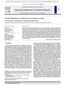
The results in Table 1 indicate that PSOCS-FNN has the best performance in almost all criteria. Table 1 also reveals that the best architecture for this function approximation problem is with S1 = 6. Figure 4 shows the convergence rates of PSO-FNN, CS-FNN, and PSOCS-FNN based on the average values of SSE in 500 iterations. It is clearly seen that during the initial iterations the convergence of the PSO-FNN was very fast; however, in the last iterations, it had almost no improvement and was trapped in local minima of the parameter space. These figures indicate that PSOCS-FNN and CS-FNN have very close results, but PSOCS-FNN is better.

Algorithms 2015, 8

302

5.2. Experiment 2: Classification Problem A popular benchmark classification problem—the Iris classification problem—was also used to test the performance of the proposed hybrid algorithm in training FNNs. The Iris dataset consists of 150 samples that can be divided into three classes, including Setosa, Versicolor, and Virginica. Each class accounts for 50 samples. All samples have four features: sepal length, sepal width, petal length, and petal width. Therefore, we used FNNs with the structure 4-S2-3 to solve this classification problem, where S2 is the number of hidden nodes with S2 = 4, 5, 6, ..., 16. In this study, 100 samples were used for training and the rest were used for testing. The search space was [−50, 50]. Every procedure was run five times successively, and then the mean values were calculated for these five results and are shown in Table 2. The results show that PSOCS-FNN outperforms PSO-FNN and CS-PSO.

Figure 4. Convergence of PSO-FNN, CS-FNN, and PSOCS-FNN in the function approximation with S1 = 3, 4, 5, 6, and 7.

Algorithms 2015, 8

303

Table 2. The comparison of the performances of the PSO-FNN, CS-FNN, and PSOCS-FNN in the Iris classification problem. Hidden Node (S2) 4

5

6

7

8

9

10

11

12

13

14

15

Algorithm PSO CS PSOCS PSO CS PSOCS PSO CS PSOCS PSO CS PSOCS PSO CS PSOCS PSO CS PSOCS PSO CS PSOCS PSO CS PSOCS PSO CS PSOCS PSO CS PSOCS PSO CS PSOCS PSO CS PSOCS

SSE 39.39494 34.353 34.21615 38.52052 33.29272 33.1576 37.81462 32.06983 31.92559 34.48936 29.9164 29.77234 33.87586 28.26575 28.14429 31.9543 26.24346 26.10769 31.13578 25.40347 25.25101 30.12397 24.69134 24.57097 28.62928 22.72357 22.57407 28.14103 21.52259 21.38662 26.44765 20.3495 20.21154 28.36295 23.45967 23.31919

Training Accuracy 0.794 0.824 0.866 0.81 0.836 0.854 0.82 0.826 0.838 0.818 0.868 0.872 0.814 0.844 0.876 0.83 0.852 0.878 0.83 0.852 0.9 0.8 0.866 0.87 0.868 0.876 0.94 0.828 0.836 0.952 0.888 0.888 0.982 0.82 0.832 0.928

Testing Accuracy 0.76 0.776 0.788 0.792 0.824 0.8 0.744 0.824 0.788 0.8 0.888 0.816 0.804 0.852 0.824 0.816 0.824 0.832 0.84 0.84 0.864 0.824 0.86 0.876 0.856 0.848 0.872 0.828 0.88 0.896 0.804 0.848 0.948 0.816 0.832 0.84

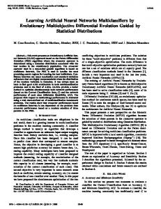
Figure 5 shows the convergence rates of PSO-FNN, CS-FNN, and PSOCS-FNN based on the average values of SSE with S2 = 10, 11, 12, 13, 14, and 15. This figure confirms that the PSOCS-FNN had a trade-off between avoiding premature convergence and exploring the whole search space for all values of hidden numbers. From Figure 6, it can be inferred that PSOCS-FNN has a better accuracy rate than PSO-FNN and CS-FNN. For the testing dataset, the best accuracy rates for PSO-FNN and

Algorithms 2015, 8

304

CS-FNN were 0.856 and 0.868, respectively; while the best accuracy rate for PSOCS-FNN was 0.948. These results prove that PSOCS-FNN is capable of solving the Iris classification problem more reliably and accurately than PSO-FNN and CS-FNN. Based on the obtained results, it can be concluded that PSOCS-FNN outperforms PSO-FNN and CS-FNN due to the capability of the proposed hybrid PSOCS algorithm.

Figure 5. Convergence of PSO-FNN, CS-FNN, and PSOCS-FNN in the Iris classification problem with S2 = 10, 11, 12, 13, 14, and 15.

Algorithms 2015, 8

305

Figure 6. Accuracy rate of PSO-FNN, CS-FNN, and PSOCS-FNN in the Iris classification problem. 6. Conclusions In this study, we proposed a hybrid PSOCS algorithm based on the PSO and CS algorithms. This algorithm combines the PSO algorithm’s strong ability regarding convergence rate and the CS algorithm’s strong ability in global search. Therefore, it has a trade-off between avoiding premature convergence and exploring the whole search space. We can get better search results using this hybrid algorithm. The PSO, CS, and PSOCS were utilized as training algorithms for FNNs. For the two benchmark problems, the comparison results showed that PSOCS-FNN outperforms PSO-FNN and CS-FNN in terms of convergence rate and being trapped in local minima. It can be concluded that the proposed hybrid PSOCS algorithm is suitable for use as a training algorithm for FNNs. The results of the present study also show the fact that a comparative analysis of different training algorithms is always supportive in enhancing the performance of a neural network. For future research, we will focus on how to apply this hybrid PSOCS algorithm to deal with more optimization problems. Acknowledgment This research was funded by the National Science Council of Taiwan under Grant No. MOST 103-2221-E-035-052.

Algorithms 2015, 8

306

Author Contributions Jeng-Fung Chen initiated the idea of the work. Quang Hung Do conducted the literature review. All of the authors developed the research design and implemented the research. The final manuscript was approved by all authors. Conflicts of Interest The authors declare no conflict of interest. References 1. 2. 3. 4. 5. 6. 7. 8. 9. 10. 11. 12. 13.

14.

Paliwal, M.; Kumar, U.A. Neural networks and statistical techniques: A review of applications. Expert Syst. Appl. 2009, 36, 2–17. Vosniakos, G.C.; Benardos, P.G. Optimizing feedforward Artificial Neural Network Architecture. Eng. Appl. Artif. Intell. 2007, 20, 365–382. Funahashi, K. On the approximate realization of continuous mappings by neural networks. Neural Netw. 1989, 2, 183–192. Norgaard, M.R.O.; Poulsen, N.K.; Hansen, L.K. Neural Networks for Modeling and Control of Dynamic Systems. A Practitioner’s Handbook; Springer: London, UK, 2000. Mat Isa, N. Clustered-hybrid multilayer perceptron network for pattern recognition application. Appl. Soft Comput. 2011, 11, 1457–1466. Homik, K.; Stinchcombe, M.; White, H. Multilayer feedforward networks are universal approximators. Neural Netw. 1989, 2, 359–366. Malakooti, B.; Zhou, Y. Approximating polynomial functions by feedforward artificial neural network: Capacity analysis and design. Appl. Math. Comput. 1998, 90, 27–52. Hush, R.; Horne, N.G. Progress in supervised neural networks. IEEE Signal Proc. Mag. 1993, 10, 8–39. Hagar, M.T.; Menhaj, M.B. Training feedforward networks with the Marquardt algorithm. IEEE Trans. Neural Netw. 1994, 5, 989–993. Adeli, H.; Hung, S.L. An adaptive conjugate gradient learning algorithm for efficient training of neural networks. Appl. Math. Comput. 1994, 62, 81–102. Zhang, N. An online gradient method with momentum for two-layer feedforward neural networks. Appl. Math. Comput. 2009, 212, 488–498. Gupta, J.N.D.; Sexton, R.S. Comparing backpropagation with a genetic algorithm for neural network training. Omega 1999, 27, 679–684. Mirjalili, S.A.; Mohd Hashim, S.Z.; Sardroudi, H.M. Training feedforward neural networks using hybrid particle swarm optimization and gravitational search algorithm. Appl. Math. Comput. 2012, 218, 11125–11137. Gori, M.; Tesi, A. On the problem of local minima in back-propagation. IEEE Trans. Pattern Anal. Mach. Intell. 1992, 14, 76–86.

Algorithms 2015, 8

307

15. Zhang, J.R.; Zhang, J.; Lock, T.M.; Lyu, M.R. A hybrid particle swarm optimization–backpropagation algorithm for feedforward neural network training. Appl. Math. Comput. 2007, 185, 1026–1037. 16. Goldberg, E. Genetic Algorithms in Search, Optimization and Machine Learning; Addison Wesley: Boston, MA, USA, 1989. 17. Kennedy, J.; Eberhart, R.C. Particle swarm optimization. In Proceedings of the 1995 IEEE International Conference on Neural Networks, Perth, Australia, 27 November–1 December 1995; Volume 4, pp. 1942–1948. 18. Dorigo, M.; Maniezzo, V.; Golomi, A. Ant system: Optimization by a colony of cooperating agents. IEEE Trans. Syst. Man Cybernet. 1996, 26, 29–41. 19. Cells, M.; Rylander, B. Neural network learning using particle swarm optimizers. In Advances in Information Science and Soft Computing; WSEAS Press: Cancun, Mexico, 2002; pp. 224–226. 20. Yang, X.S.; Deb, S. Cuckoo search via Lévy flights. In Proceedings of the IEEE World Congress on Nature and Biologically Inspired Computing (NaBIC 2009), Coimbatore, India, 9–11 December 2009; pp. 210–214. 21. Yang, X.S.; Deb, S. Engineering Optimisation by Cuckoo Search. Int. J. Math. Model. Numer. Optim. 2010, 1, 330–343. 22. Valian, E.; Mohanna, S.; Tavakoli, S. Improved Cuckoo Search Algorithm for Feedforward Neural Network Training. Int. J. Artif. Intell. Appl. 2009, 2, 36–43. 23. Ouaarab, A.; Ahiod, B.; Yang, X.S. Discrete cuckoo search algorithm for the travelling salesman problem. Neural Comput. Appl. 2014, 24, 1659–1669. 24. Zhou, Y.; Zheng, H. A novel complex valued Cuckoo Search algorithm. Sci. World J. 2013. doi:10.1155/2013/597803. 25. Li, L.K.; Shao, S.; Yiu, K.F.C. A new optimization algorithm for single hidden layer feedforward neural networks. Appl. Soft Comput. 2013, 13, 2857–2862. 26. Kiranyaz, S.; Ince, T.; Yildirim, A.; Gabbouj, M. Evolutionary artificial neural networks by multi-dimensional particle swarm optimization. Neural Netw. 2009, 22, 1448–1462. 27. Mirjalili S.; Hashim, S.Z.M. A New Hybrid PSOGSA Algorithm for Function Optimization. In Proceedings of the International Conference on Computer and Information Application (ICCIA 2010), Tianjin, China, 3–5 December 2010; pp. 374–377. 28. Rashedi, E.; Nezamabadi-pour, H.; Saryazdi, S. GSA: A Gravitational Search Algorithm. Inf. Sci. 2009, 179, 2232–2248. 29. Civicioglu, P. Transforming Geocentric Cartesian Coordinates to Geodetic Coordinates by Using Differential Search Algorithm. Comput. Geosci. 2012, 46, 229–247. 30. Civicioglu, P. Artificial cooperative search algorithm for numerical optimization problems. Inf. Sci. 2013, 229, 58–76. 31. Civicioglu, P.; Besdok, E. A conceptual comparison of the cuckoo-search, particle swarm optimization, differential evolution and artificial bee colony algorithms. Artif. Intell. Rev. 2013, 39, 315–346. 32. Civicioglu, P. Backtracking Search Optimization Algorithm for numerical optimization problems. Appl. Math. Comput. 2013, 219, 8121–8144.

Algorithms 2015, 8

308

33. Lai, X.; Zhang, M. An efficient ensemble of GA and PSO for real function optimization. In Proceedings of 2nd IEEE International Conference on Computer Science and Information Technology, Beijing, China, 8–11 August 2009; pp. 651–655. 34. Esmin, A.A.A.; Lambert-Torres, G.; Alvarenga, G.B. Hybrid Evolutionary Algorithm Based on PSO and GA mutation. In Proceeding of the Sixth International Conference on Hybrid Intelligent Systems (HIS 06), Auckland, New Zealand, 13–15 December 2006; p. 57. 35. Li, L.; Xue, B.; Niu, B.; Tan, L.; Wang, J. A Novel PSO-DE-Based Hybrid Algorithm for Global Optimization. Lect. Notes Comput. Sci. 2007, 785–793. 36. Holden, N.; Freitas, A.A. A Hybrid PSO/ACO Algorithm for Discovering Classification Rules in Data Mining. J. Artif. Evolut. Appl. 2008, doi:10.1155/2008/316145. 37. Ghodrati, A.; Lotfi, S. A Hybrid CS/PSO Algorithm for Global Optimization, Intelligent Information and Database Systems. Lect. Notes Comput. Sci. Vol. 2012, 7198, 89–98. 38. Yang, X.S.; Deb, S. Cuckoo Search: Recent Advances and Applications. Neural Comput. Appl. 2014, 24, 169–174. 39. Caruana, R.; Lawrence, S.; Giles, C.L. Overfitting in neural networks: Backpropagation, conjugate gradient, and early stopping. In Advances Neural Information Processing Systems; Leen, T.K., Dietterich, T.G., Tresp, V., Eds.; MIT Press: Denver, CO, USA, 2000; Volume 13, pp. 402–408. © 2015 by the authors; licensee MDPI, Basel, Switzerland. This article is an open access article distributed under the terms and conditions of the Creative Commons Attribution license (http://creativecommons.org/licenses/by/4.0/).