Training Support Vector Machines: an Application to Face ... - CiteSeerX

Training Support Vector Machines: an Application to Face Detection (To appear in the Proceedings of CVPR'97, June 17-19, 1997, Puerto Rico.) y

Edgar Osunay? Robert Freund? Federico Girosiy Center for Biological and Computational Learning and ?Operations Research Center Massachusetts Institute of Technology Cambridge, MA, 02139, U.S.A.

Abstract

We investigate the application of Support Vector Machines (SVMs) in computer vision. SVM is a learning technique developed by V. Vapnik and his team (AT&T Bell Labs.) that can be seen as a new method for training polynomial, neural network, or Radial Basis Functions classi ers. The decision surfaces are found by solving a linearly constrained quadratic programming problem. This optimization problem is challenging because the quadratic form is completely dense and the memory requirements grow with the square of the number of data points. We present a decomposition algorithm that guarantees global optimality, and can be used to train SVM's over very large data sets. The main idea behind the decomposition is the iterative solution of sub-problems and the evaluation of optimality conditions which are used both to generate improved iterative values, and also establish the stopping criteria for the algorithm. We present experimental results of our implementation of SVM, and demonstrate the feasibility of our approach on a face detection problem that involves a data set of 50,000 data points.

1 Introduction

In recent years problems such as object detection or image classi cation have received an increasing amount of attention in the computer vision community. In many cases these problems involve \concepts" (like \face", or \people") that cannot be expressed in terms of a small and meaningful set of features, and the only feasible approach is to learn the solution from a set of examples. The complexity of these problems is often such that an extremely large set of examples is needed in order to learn the task with the desired accuracy. Moreover, since it is not known what are the relevant features of the problem, the data points usually belong to some high-dimensional space (for example an image may be represented by its grey level values, eventually ltered with a bank of lters, or by a dense vector eld that puts it in correspondence with a certain prototypical image). Therefore, there is a need for general purpose pattern recognition techniques that can handle large data sets (105 ? 106 data points) in high dimensional spaces (102 ? 103 ). In this paper we concentrate on the Support Vector Machine (SVM), a pattern classi cation algorithm recently developed by V. Vapnik and his team at AT&T

Bell Labs. [1, 3, 4, 12]. SVM can be seen as a new way to train polynomial, neural network, or Radial Basis Functions classi ers. While most of the techniques used to train the above mentioned classi ers are based on the idea of minimizing the training error, which is usually called empirical risk, SVMs operate on another induction principle, called structural risk minimization, which minimizes an upper bound on the generalization error. From the implementation point of view, training a SVM is equivalent to solving a linearly constrained Quadratic Programming (QP) problem in a number of variables equal to the number of data points. This problem is challenging when the size of the data set becomes larger than a few thousands. In this paper we show that a large scale QP problem of the type posed by SVM can be solved by a decomposition algorithm: the original problem is replaced by a sequence of smaller problems, that is proved to converge to the global optimum. In order to show the applicability of our approach we used SVM as the core classi cation algorithm in a face detection system. The problem that we have to solve involves training a classi er to discriminate between face and non-face patterns, using a data set of 50,000 points. The plan of the paper is as follows: in the rest of this section we brie y introduce the SVM algorithm and its geometrical interpretation. In section 2 we present our solution to the problem of training a SVM and our decomposition algorithm. In section 3 we present our application to the face detection problem, and in section 4 we summarize our results.

1.1 Support Vector Machines

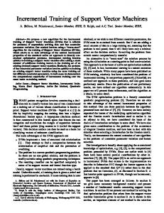
In this section we brie y sketch the SVM algorithm and its motivation. A more detailed description of SVM can be found in [12] (chapter 5) and [4]. We start from the simple case of two linearly separable classes. We assume that we have a data set D = f(xi ; yi)g`i=1 of labeled examples, where yi 2 f?1; 1g, and we wish to determine, among the in nite number of linear classifers that separate the data, which one will have the smallest generalization error. Intuitively, a good choice is the hyperplane that leaves the maximum margin between the two classes, where the margin is de ned as the sum of the distances of the hyperplane from the closest point of the two classes (see gure 1). If the two classes are non-separable we can still look for

(a)

(b)

Figure 1: (a) A Separating Hyperplane with small

margin. (b) A Separating Hyperplane with larger margin. A better generalization capability is expected

from (b).

the hyperplane that maximizes the margin and that minimizes a quantity proportional to the number of misclassi cation errors. The trade o between margin and misclassi cation error is controlled by a positive constant C that has to be chosen beforehand. In this case it can be shown that the solution P to this problem is a linear classi er f (x) = sign( `i=1 i yi xT xi + b) whose coecents i are the solution of the following QP problem: Minimize W ()  subject to

= ?T 1 + 21 T D

(1) T y = 0  ? C1  0 ? 0 where ()i = i , (1)i = 1 and Dij = yi yj xTi xj . It

turns out that only a small number of coecients i are dierent from zero, and since every coecient corresponds to a particular data point, this means that the solution is determined by the data points associated to the non-zero coecients. These data points, that are called support vectors, are the only ones which are relevant for the solution of the problem: all the other data points could be deleted from the data set and the same solution would be obtained. Intuitively, the support vectors are the data points that lie at the border between the two classes. Their number is usually small, and Vapnik showed that it is proportional to the generalization error of the classi er. Since it is unlikely that any real life problem can actually be solved by a linear classi er, the technique has to be extended in order to allow for non-linear decision surfaces. This is easily done by projecting the original set of variables x in a higher dimensional feature space: x 2 Rd ) z(x)  (1(x); : : : ; n(x)) 2 Rn and by formulating the linear classi cation problem in the featurePspace. The solution will have the form f (x) = sign( `i=1 i yi zT (x)z(xi ) + b), and therefore will be nonlinear in the original input variables. One has to face at this point two problems: 1) the choice of the features i (x), which should be done in a way

that leads to a \rich" class of decision surfaces; 2) the computation of the scalar product zT (x)z(xi ), which can be computationally prohibitive if the number of features n is very large (for example in the case in which one wants the feature space to span the set of polynomials in d variables the number of features n is exponential in d). A possible solution to this problems consists in letting n go to in nity and make the following choice: z(x)  (p1 1 (x); : : :; pi i (x); : : :) where i and i are the eigenvalues and eigenfunctions of an integral operator whose kernel K (x; y) is a positive de nite symmetric function. With this choice the scalar product in the feature space becomes particularly simple because:

zT (x)z(y) =

1 X  i=1

i i (x) i (y) = K (x; y)

where the last equality comes from the MercerHilbert-Schmidt theorem for positive de nite functions (see [8], pp. 242{246). The QP problem that has to be solved now is exactly the same as in eq. (1), with the exception that the matrix D has now elements Dij = yi yj K (xi ; xj ). As a result of this choice, P the SVM classi er has the form: f (x) = sign( `i=1 i yi K (x; xi ) + b). In table (1) we list some choices of the kernel function proposed by Vapnik: notice how they lead to well known classi ers, whose decision surfaces are known to have good approximation properties. Kernel Function Type of Classi er K (x; xi ) = exp(?kx ? xi k2) Gaussian RBF K (x; xi ) = (xT xi + 1)d Polynomial of degree d K (x; xi ) = tanh(xT xi ? ) Multi Layer Perceptron Table 1: Some possible kernel functions and the type of decision surface they de ne

2 Training a Support Vector Machine

As mentioned before, training a SVM using large data sets (above  5,000 samples) is a very dicult problem to approach without some kind of problem decomposition. To give an idea of some memory requirements, an application like the one described in section 3 involves 50,000 training samples, and this amounts to a quadratic form whose matrix D has 2:5
109 entries that would need, using an 8-bytes oating point representation, 20 Gigabytes of memory. In order to solve the training problem eciently, we take explicit advantage of the geometrical interpretation introduced in Section 1.1, in particular, the expectation that the number of support vectors will be very small, and therefore that many of the components of  will be zero. In order to decompose the original problem, one can think of solving iteratively the system given by (1), but keeping xed at zero level those components

i associated with data points that are not support

vectors, and therefore only optimizing over a reduced set of variables. To convert the previous description into an algorithm we need to specify: 1. Optimality Conditions: These conditions allow us to decide computationally, if the problem has been solved optimally at a particular iteration of the original problem. Section 2.1 states and proves optimality conditions for the QP given by (1). 2. Strategy for Improvement: If a particular solution is not optimal, this strategy de nes a way to improve the cost function and is frequently associated with variables that violate optimality conditions. This strategy will be stated in section 2.2. After presenting optimality conditions and a strategy for improving the cost function, section 2.3 introduces a decomposition algorithm that can be used to solve large database training problems, and section 2.4 reports some computational results obtained with its implementation.

2.1 Optimality Conditions

The QP problem we have to solve is the following: Minimize W ()  subject to

= ?T 1 + 12 T D

(D)i ? 1 + yi = 0

Using the results in [4] and [12] one can easily show that when  is strictly between 0 and C the following equality holds: ` X y (  y K (x ; x ) + b) = 1 i

(3)

=0

0 0

j j

(5)

i j

(D)i =

X`  y y K (x ; x )= y X`  y K (x ; x ) j j i

j =1

i j

i

j =1

j j

i j

and combining this expression with (5) and (4) we immediately obtain that  = b. 2. Case: i = C From the rst three equations of the KT conditions we have: (D)i ? 1 + i + yi = 0

(6)

By de ning

() () () (2) where , T = (1 ; : : :; `) and T = (1; : : :; `) are the associated Kuhn-Tucker multipliers. Since D is a positive semi-de nite matrix ( the kernel function used is positive de nite ), and the constraints in (2) are linear, the Kuhn-Tucker, (KT) conditions are necessary and sucient for optimality. The KT conditions are as follows: rW () +  ?  + y = 0 TT ( ? C 1) =0   =0

0 0

j =1

Noticing that

T y = 0  ? C1  0 ? 0

  T y  ? C1 ?

(4)

In order to derive further algebraic expressions from the optimality conditions (3), we assume the existence of some i such that 0 < i < C , and consider the three possible values that each component of  can have: 1. Case: 0 < i < C From the rst three equations of the KT conditions we have:

g(xi ) =

X`  y K (x ; x ) + b j =1

j j

(7)

i j

and noticing that ` X (D) = y  y K (x ; x ) = y (g(x ) ? b) i

i

j =1

j j

i j

i

i

we conclude from equation (6) that yi g(xi )  1

(8)

(where we have used the fact that  = b and required the KT multiplier i to be positive). 3. Case: i = 0 From the rst three equations of the KT conditions we have: (D)i ? 1 ? i + yi = 0

(9)

By applying a similar algebraic manipulation as the one described for case 2, we obtain yi g(xi )  1

(10)

2.2 Strategy for Improvement

The optimality conditions derived in the previous section are essential in order to devise a decomposition strategy that takes advantage of the expectation that most i 's will be zero, and that guarantees that at every iteration the objective function is improved. In order to accomplish this goal we partition the index set in two sets B and N in such a way that the optimality conditions hold in the subproblem de ned only for the variables in the set B , which is called the working set. Then we decompose  in two vectors B and N and set N = 0. Using this decomposition the following statements are clearly true:  We can replace i = 0, i 2 B , with j = 0, j 2 N , without changing the cost function or the feasibility of both the subproblem and the original problem.  After such a replacement, the new subproblem is optimal if and only if yj g(xj )  1. This follows from equation (10) and the assumption that the subproblem was optimal before the replacement was done. The previous statements lead to the following proposition:

Proposition 2.1 Given an optimal solution of a subproblem de ned on B , the operation of replacing i = 0, i 2 B , with j = 0, j 2 N , satisfying yj g(xj )
0 such that p ?  > 0, for  2 (0; ). Notice also that g(xp ) = yp . Now, consider  =  + ej ? ep , where ej and ep are the j -th and p-th unit vectors, and notice that the pivot operation can be handled implicitly by letting  > 0 and by holding i = 0. The new cost function W () can be written as: 1 T D 2 1 T = ? 1 + 2 T D + T D(ej ? ep ) + + 12 (ej ? ep )T D(ej ? ep ) = W () +  [(g(xj ) ? b)yj ? 1 + byp ] + 2 + 2 [K (xj ; xj )+ K (xp ; xp ) ? 2yp yj K (xp ; xj )]

W ()= ?T 1 +

= W () +  [g(xj )yj ? 1] + 2 [K (xj ; xj ) +K (xp ; xp) ? 2yp yj K (xp ; xj )] Therefore, since g(xj )yj < 1, by choosing  small enough we have W () < W (). 2

2.3 The Decomposition Algorithm

Suppose we can de ne a xed-size working set B , such that jB j  `, and it is big enough to contain all support vectors (i > 0), but small enough such that the computer can handle it and optimize it using some solver. Then the decomposition algorithm can be stated as follows: 1. Arbitrarily choose jB j points from the data set. 2. Solve the subproblem de ned by the variables in B. 3. While there exists some j 2 N , such that g(xj )yj < 1, replace i = 0, i 2 B , with j = 0 and solve the new subproblem. Notice that, according to (2.1), this algorithm will strictly improve the objective function at each iteration and therefore will not cycle. Since the objective function is bounded (W () is convex quadratic and the feasible region is bounded), the algorithm must converge to the global optimal solution in a nite number of iterations. Figure 2 gives a geometric interpretation of the way the decomposition algorithm allows the rede nition of the separating surface by adding points that violate the optimality conditions.

(a)

(b)

Figure 2: (a) A sub-optimal solution where the non lled points have  = 0 but are violating optimality conditions by being inside the 1 area. (b) The decision surface is rede ned. Since no points with  = 0 are inside the 1 area, the solution is optimal. Notice that the size of the margin has decreased, and the shape of the decision surface has changed.

2.4 Implementation and Results

We have implemented the decomposition algorithm using MINOS 5.4 as the solver of the sub-problems. For information on MINOS 5.4 see [7]. The computational results that we present in this section have been obtained using real data from our Face Detection System, which is described in Section 3. Figures 3a and 3b show the training time and the number of support vectors obtained when training the system with 5,000, 10,000, 20,000, 30,000, 40,000, 49,000, and 50,000 data points. The discontinuity in the graphs between 49,000 and 50,000 data points is due to the fact that the last 1,000 data points were collected

3 SVM Application: Face Detection in Images

This section introduces a Support Vector Machine application for detecting vertically oriented and unoccluded frontal views of human faces in grey level images. It handles faces over a wide range of scales and works under dierent lighting conditions, even with moderately strong shadows. The face detection problem can be de ned as follows: given as input an arbitrary image, which could be a digitized video signal or a scanned photograph, determine whether or not there are any human faces in the image, and if there are, return an encoding of their location. Face detection as a computer vision task has many applications. It has direct relevance to the face recognition problem, because the rst important step of a fully automatic human face recognizer is usually locating faces in an unknown image. Face detection also has potential application in human-computer interfaces, surveillance systems, census systems, etc. From the standpoint of this paper, face detection is interesting because it is an example of a natural and challenging problem for demonstrating and testing the potentials of Support Vector Machines. There are many other object classes and phenomena in the real world that share similar characteristics, for example, tumor anomalies in MRI scans, structural defects in manufactured parts, etc. A successful and general

5

1000

4.5 900 4 Number of Support Vectors

Time (hours)

3.5 3 2.5 2 1.5

800

700

600

500

1 400 0.5

(a)

0 0

0.5

1

1.5

2

2.5 3 3.5 Number of Samples

4

4.5

5 4

x 10

(b)

300 0

0.5

1

1.5

2

2.5 3 3.5 Number of Samples

4

4.5

5 4

x 10

16

5 4.5

14

4 Number of Global Iterations

12

3.5 Time (hours)

in the last phase of bootstrapping of the Face Detection System (see section 3.2). This means that the last 1,000 data points are points which were misclassi ed by the previous version of the classi er, which was already quite accurate, and therefore points likely to be on the border between the two classes and therefore very hard to classify. Figure 3c shows the relationship between the training time and the number of support vectors. Notice how this curve is much smoother than the one in gure 3a. This means that the number of training data is not a good predictor of training time, which depends more heavily on the number of support vectors: one could add a large number of data points without increasing much the training time if the new data points do not contain new support vectors. In gure 3d we report the number of global iterations (the number of times the decomposition algorithm calls the solver) as a function of support vectors. Notice the jump from 11 to 15 global iterations as we go from 49,000 to 50,000 samples adding 1,000 \dicult" data points. The memory requirements of this technique are quadratic in the size of the working set B . For the 50,000 points data set we used a working set of 1,200 variables, that ended up using only 25Mb of RAM. However, a working set of 2,800 variables will use approximately 128Mb of RAM. Therefore, the current technique can deal with problems with less than 2,800 support vectors (actually we empirically found that the working set size should be about 20% larger than the number of support vectors). In order to overcome this limitation we are implementing an extension of the decomposition algorithm that let us deal with very large numbers of support vectors (say 10,000).

3 2.5 2 1.5

10

8

6

4

1 2

(c)

0.5 0 300

400

500

600 700 Number of Support Vectors

800

900

1000

(d)

0 0

0.5

1

1.5

2

2.5 3 3.5 Number of Samples

4

4.5

5

Figure 3: (a) Training Time on a SPARC station-20 vs. number of samples; (b)Number of Support Vectors vs. number of samples; (c) Training Time on a SPARCstation-20 vs. Number of Support Vectors. Notice how the number of support vectors is a better indicator of the increase in training time than the number of samples alone; (d) Number of global iterations performed by the algorithm. methodology for nding faces using SVM's should generalize well for other spatially well-de ned pattern and feature detection problems. It is important to remark that face detection, like most object detection problems, is a dicult task due to the signi cant pattern variations that are hard to parameterize analytically. Some common sources of pattern variations are facial appearance, expression, presence or absence of common structural features, like glasses or a moustache, light source distribution, shadows, etc. The system works by scanning an image for facelike patterns at many possible scales and uses a SVM as its core classi cation algorithms to determine the appropriate class (face/non-face).

3.1 Previous Systems

The problem of face detection has been approached with dierent techniques in the last few years. This techniques include Neural Networks [2, 9, 11], detection of face features and use of geometrical constraints [13], density estimation of the training data [6], labeled graphs [5] and clustering and distribution-based modeling [10]. Out of all these previous works, the results of Sung and Poggio [10], and Rowley et al. [9] re ect systems with very high detection rates and low false positive rates. Sung and Poggio use clustering and distance metrics to model the distribution of the face and non-face manifold, and a Neural Network to classify a new pattern given the measurements. The key of the quality of their result is the clustering and use of combined

4

x 10

Mahalanobis and Euclidean metrics to measure the distance from a new pattern and the clusters. Other important features of their approach is the use of nonface clusters, and the use of a bootstrapping technique to collect important non-face patterns. One drawback of this technique is that it does not provide a principled way to choose some important free parameters like the number of clusters it uses. Similarly, Rowley et al. have used problem information in the design of a retinally connected Neural Network that is trained to classify faces and non-faces patterns. Their approach relies on training several NN emphasizing subsets of the training data, in order to obtain dierent sets of weights. Then, dierent schemes of arbitration between them are used in order to reach a nal answer. Our approach to face detection with SVM uses no prior information in order to obtain the decision surface, so that this technique could be used to detect other kind of objects in digital images.

3.2 The SVM Face Detection System

This system detects faces by exhaustively scanning an image for face-like patterns at many possible scales, by dividing the original image into overlapping subimages and classifying them using a SVM to determine the appropriate class (face/non-face). Multiple scales are handled by examining windows taken from scaled versions of the original image. More speci cally, this system works as follows: 1. A database of face and non-face 19  19 = 361 pixel patterns, assigned to classes +1 and -1 respectively, is used to train a SVM with a 2nddegree polynomial as kernel function and an upper bound C = 200. 2. In order to compensate for certain sources of image variation, some preprocessing of the data is performed:  Masking: A binary pixel mask is used to remove some pixels close to the boundary of the window pattern allowing a reduction in the dimensionality of the input space to 283. This step is important in the reduction of background patterns that introduce unnecessary noise in the training process.  Illumination gradient correction: A best- t brightness plane is subtracted from the unmasked window pixel values, allowing reduction of light and heavy shadows.  Histogram equalization: A histogram equalization is performed over the patterns in order to compensate for dierences in illumination brightness, dierent cameras response curves, etc. 3. Once a decision surface has been obtained through training, the run-time system is used over images that do not contain faces, and misclassi cations are stored so they can be used as negative examples in subsequent training phases. Images of landscapes, trees, buildings, rocks, etc., are good sources of false positives due to the many

dierent textured patterns they contain. This bootstrapping step, which was successfully used by Sung and Poggio [10] is very important in the context of a face detector that learns from examples because:  Although negative examples are abundant, negative examples that are useful from a learning point of view are very dicult to characterize and de ne.  The two classes, face and non-face are not equally complex since the non-face class is broader and richer, and therefore needs more examples in order to get an accurate de nition that separates it from the face class. Figure 4 shows an image used for bootstrapping with some misclassi cations, that were later used as non-face examples. 4. After training the SVM, we incorporate it as the classi er in a run-time system very similar to the one used by Sung and Poggio [10] that performs the following operations:  Re-scale the input image several times.  Cut 1919 window patterns out of the scaled image.  Preprocess the window using masking, light correction and histogram equalization.  Classify the pattern using the SVM.  If the pattern is a face, draw a rectangle around it in the output image.

Figure 4: Some false detections obtained with the rst version of the system. This false positives were later used as non-face examples in the training process

3.2.1 Experimental Results

To test the run-time system, we used two sets of images. The set A, contained 313 high-quality images with one face per image. The set B, contained 23 images of mixed quality, with a total of 155 faces. Both

sets were tested using our system and the one by Sung and Poggio [10]. In order to give true meaning to the number of false positives obtained, it is important to state that set A involved 4,669,960 pattern windows, while set B 5,383,682. Table 2 shows a comparison between the 2 systems. At run-time the SVM system is approximately 30 times faster than the system of Sung and Poggio. One reason for that is the use of a technique introduced by C. Burges [3] that allows to replace a large numbers of support vectors with a much smaller number of points (which are not necessarily data points), and therefore to speed up the run time considerably. In gure 5 we report the result of our system on some test images. Notice that the system is able to handle, up to a small degree, non-frontal views of faces. However, since the database does not contain any example of occluded faces the system usually misses partially covered faces, like the ones in the bottom picture of gure 5. The system can also deal with some degree of rotation in the image plane, since the data base contains a number of \virtual" faces that were obtained by rotating some face example of up to 10 degrees. In gure 6 we report some of the support vectors we obtained, both for face and non-face patterns. We represent images as points in a ctitious two dimensional space and draw an arbitrary boundary between the two classes. Notice how we have placed the support vectors at the classi cation boundary, accordingly with their geometrical interpretation. Notice also how the non-face support vectors are not just random non-face patterns, but are non-face patterns that are quite similar to faces.

SVM Sung et al.

Test Set A Detect False Rate Alarms 97.1 % 4 94.6 % 2

Test Set B Detect False Rate Alarms 74.2% 20 74.2% 11

Table 2: Performance of the SVM face detection system

4 Summary and Conclusions

In this paper we have presented a novel decomposition algorithm that can be used to train Support Vector Machines on large data sets (say 50,000 data points). The current version of the algorithm can deal with about 2,500 support vectors on a machine with 128 Mb of RAM, but an implementation of the technique currently under development will be able to deal with much larger number of support vectors (say about 10,000) using less memory. We demonstrated the applicability of SVM by embedding SVM in a face detection system which performs comparably to other state-of-the-art systems. There are several reasons for which we have been investigating the use of SVM. Among them, the fact that SVMs are very well founded from the mathematical point of view, being an approximate implementation of the Structural Risk Minimization induction principle. The only free parameters of SVMs are the positive constant C and the parameter associated to the kernel K (in our case

Figure 5: Results from our Face Detection system

NON-FACES

[2] [3] [4] [5] [6]

FACES

Figure 6: In this picture circles represent face patterns and squares represent non-face patterns. On the border between the two classes we represented some of the support vectors found by our system. Notice how some of the non-face support vectors are very similar to faces. the degree of the polynomial). The technique appears to be stable with respect to variations in both parameters. Since the expected value of the ratio between the number of support vectors and the total number of data points is an upper bound on the generalization error, the number of support vector gives us an immediate estimate of the diculty of the problem. SVMs handle very well high dimensional input vectors, and therefore their use seem to be appropriate in computer vision problems in which it is not clear what the features are, allowing the user to represent the image as a (possibly large) vector of grey levels 1 .

Acknowledgements

The authors would like to thank Tomaso Poggio, Vladimir Vapnik, Michael Oren and Constantine Papageorgiou for useful comments and discussion.

References

[1] B.E. Boser, I.M. Guyon, and V.N. Vapnik. A training algorithm for optimal margin classi er. In Proc. 5th

1 This paper describes research done within the Center for Biological and Computational Learning in the Department of Brain and Cognitive Sciences and at the Arti cial Intelligence Laboratory at MIT. This research is sponsored by a grant from NSF under contract ASC-9217041 (this award includes funds from ARPA provided under the HPCC program), by a grant from ARPA/ONR under contract N00014-92-J-1879 and by a MURI grant under contract N00014-95-1-0600.Additional support is provided by Daimler-Benz, Sumitomo Metal Industries, and Siemens AG. Edgar Osuna was supported by Fundacion Gran Mariscal de Ayacucho.

[7] [8] [9] [10] [11] [12] [13]

ACM Workshop on Computational Learning Theory, pages 144{152, Pittsburgh, PA, July 1992. G. Burel and D. Carel. Detection and localization of faces on digital images. Pattern Recognition Letters, 15:963{967, 1994. C.J.C. Burges. Simpli ed support vector decision rules. In International Conference on Machine Learning, pages 71{77. 1996. C. Cortes and V. Vapnik. Support vector networks. Machine Learning, 20:1{25, 1995. N. Kruger, M. Potzsch, and C. v.d. Malsburg. Determination of face position and pose with learned representation based on labled graphs. Technical Report 96-03, Ruhr-Universitat, January 1996. B. Moghaddam and A. Pentland. Probabilistic visual learning for object detection. Technical Report 326, MIT Media Laboratory, June 1995. B. Murtagh and M. Saunders. Large-scale linearly constrained optimization. Mathematical Programming, 14:41{72, 1978. F. Riesz and B. Sz.-Nagy. Functional Analysis. Ungar, New York, 1955. H. Rowley, S. Baluja, and T. Kanade. Human face detection in visual scenes. Technical Report CMUCS-95-158R, School of Computer Science, Carnegie Mellon University, November 1995. K. Sung and T. Poggio. Example-based Learning for View-based Human Face Detection. A.I. Memo 1521, MIT A.I. Lab., December 1994. R. Vaillant, C. Monrocq, and Y. Le Cun. Original approach for the localisation of objects in images. IEEE Proc. Vis. Image Signal Process., 141(4), August 1994. V. Vapnik. The Nature of Statistical Learning Theory. Springer, New York, 1995. G. Yang and T. Huang. Human face detection in a complex background. Pattern Recognition, 27:53{63, 1994.