mizing the robot trajectories for o -line programming. Thus, improved set ... conveniently in combination with computer-aided robotics (CAR) tools and current.
Accepted for publication in Optimization (1999).
TRAJECTORY OPTIMIZATION OF INDUSTRIAL ROBOTS WITH APPLICATION TO COMPUTER-AIDED ROBOTICS AND ROBOT CONTROLLERS
ALEXANDER HEIM and OSKAR VON STRYK Department of Mathematics, Technische Universitat Munchen, D-80290 Munchen, Germany, http://www-m2.ma.tum.de/ The workcycle time in automated car manufacturing lines can be reduced by optimizing the robot trajectories for o�-line programming. Thus, improved set points for the on-line robot controller are obtained. In this paper, direct transcription methods are described for solving the constrained trajectory optimization problems by using full dynamic robot models. The optimization methods can be used conveniently in combination with computer-aided robotics (CAR) tools and current robot controllers. This is demonstrated by simulation and experimental results for an ABB IRB 6400 industrial robot. Keywords: state constrained optimal control; direct transcription method; optimal robot trajectories; on-line robot control; computer-aided robotics
1 Introduction An automated manufacturing line in automotive industry consists of workcells with several robotic manipulators. The reduction of the overall workcycle time needed per car is of great economic importance for improving productivity. Virtual manufacturing software must be used for rapidly designing each workcell and planning the tasks of each robot. For example, CATIA{ Robotics, IGRIP, ROBCAD, or SILMA{CimStation are graphicsbased interactive simulation systems for planning and o�-line programming of robot cells by numerical simulation of the kinematic and dynamic behavior of each robot. Here, we investigate a subproblem of the optimal design problem of the whole production process: the computation and imple-
2
A. Heim, O. von Stryk
mentation of optimal robot movements. The best robot trajectories can be obtained by trajectory optimization using full dynamic models. Tailored dynamic optimization methods based on direct transcription of optimal control problems rapidly compute openloop optimal trajectories which serve as set-points for the on-line robot controller. However, for application in industry, the mathematical optimization must be connected to currently used virtual manufacturing software and must be compatible with current robot controllers. In this paper, the potential and the di�culties of mathematical trajectory optimization methods are demonstrated by computational and experimental results for an ABB IRB 6400 robot [12], the corresponding S4 robot controller [13], and the ROBCAD computer-aided robotics tool [14].
1.1 Industrial Robotic System
Figure 1. Structure of a typical industrial robotic system.
An industrial robotic system as shown in Figure 1 consists of { a multi-purpose robotic manipulator consisting of mechanical bodies linked by rotational or prismatic joints which are controlled by motors, { an exchangeable work tool attached to the end e�ector, and { a control unit in an external cabinet which is usually placed in a remote area, away from the robot, and connected to the
Trajectory Optimization of Industrial Robotic Systems
3
manipulator by cables, plus a control panel for optional manual operation. For a high simulation accuracy of fast robot movements, proper dynamic models must be considered for the manipulator and for the on-line robot controller.
1.2 Kinematic Simulation
Geometric robot models describe the position and the orientiation of the robot arms and of the end e�ector depending on the joint variables [4]. The kinematic simulation of robots within a workcell is important for the detection of possible collisions.
1.3 Dynamic Simulation
Figure 2. The six joints of the ABB IRB 6400 series of industrial robots [12].
Industrial robots must act very fast. Thus, a dynamic model must take into account the e�ects of inertia, Coriolis, centrifugal, gravitational, and frictional forces. Therefore, the robot is described by rigid mechanical bodies that are interconnected by joints that can move or articulate in two or three dimensions. The equations of motion can be derived (almost) automatically using either advanced multibody system (MBS) tools [16] or symbolic computation tools. Usually, the robotic MBS has a tree structure. In this case, the equations of motion can be formulated as a semi-implicit
4
A. Heim, O. von Stryk
system of second order di�erential equations using global minimal coordinates (see Equation (1)). Here, we consider an industrial robot of the ABB IRB 6400 series consisting of six controllable, rotational joints (Figure 2). The rst three joints determine the position and the last three joints the orientation of the end e�ector. Several robot variants of this series are available for di�erent applications [9,12]. We consider the model IRB 6400/2.8{120 with a maximum range of 2.80 m, a maximum payload of 120 kg, and a weight of about 2 t. The design of this robot has some specialities. A supplementary load can be place on the rst arm and a strut links the motions of the second and third axis. Also, the second axis has a pneumatic weight compensation. A suitable dynamic robot model was not available. Therefore, the equations of motions had to be derived explicitly in [6] for the rst three degrees-of-freedom (DOF) q = (q1 ; q2; q3 )T : IR ! IR3 () 2 1( ) 3 1( )
() 2 2( ) 3 2( )
! !
() 2 3( ) 3 3( )
q1
M1;1 q
M1;2 q
M1;3 q
M ;
q
M ;
q
M ;
q
q2
M ;
q
M ;
q
M ;
q
q3
=
!
u1 u2 u3
+
!
( _) 2 ( _) 3 ( _)
h1
q; q
h
q; q
h
q; q
?
!
sign( _1 ) 2 sign( _2 ) : (1) 3 sign( _3 )
r1
q
r
q
r
q
Hereby, a generalized arm has been assumed with constant values for q4 , q5, q6 . The Lagrangian formalism and symbolic computation with Maple V [3] has been used to derive Equation (1) explicitly as a Fortran subroutine [6]. The mass matrix M : IR3 ! IR3�3 is symmetric and positive de nite; the vector of actuator torques u = (u1 ; u2 ; u3 )T : IR ! IR3 is the control variable; h : IR6 ! IR3 denotes the moments resulting from Coriolis, centrifugal, and gravitational forces; r denotes the constant Coulomb friction coe�cient of the i-th joint. The discontinuities caused by the friction model can be smoothed by an appropriate approximation such as r arctan(c q_ )=(�=2) with a suitable constant c . Besides the derivation of the dynamic equations, dynamical parameters such as mass, center of mass, inertia and friction coe�cients must be determined for each body. Here, the values are taken from [12] and the corresponding RRS data sheet (see Section 4). Usually, the identi cation of dynamical parameters for model calibration on the shop oor is a di�cult task [1,7,18]. i
i
i
i
i
Trajectory Optimization of Industrial Robotic Systems
5
The angles of rotation and the angular velocities of each joint are constrained by lower and upper bounds [12] q min � q (t) � q max; q_ min � q_ (t) � q_ max ; i = 1; : : : ; 6: (2) i;
i
i;
i;
i
i;
The torque-strut on the second axis links the motions of the second and third axis resulting in another constraint
?65 [deg] � q2 ? q3 � +65 [deg]:
(3)
Also, the velocity of the tool center point (TCP)is constrained by
jvelocityTCP (t)j � +5:0 m/s:
(4)
2 Optimal O�-line Programming Using Mathematical Trajectory Optimization Here, we investigate point-to-point (PTP) trajectories from a given initial position A to a nal position B A: q(0) = q0 ; q_(0) = q_0 ; B: q(t ) = q ; q_(t ) = q_ ; f
f
f
f
(5)
with given constants q0, q_0 , q , q_ 2 IR3 . Usually, stationary boundary conditions are considered, i. e., q_0 = q_ = 0. PTP trajectories arise in material handling or spot-welding. Other trajectories require path following, e. g., for glueing or arc welding. The control variable u(t), 0 � t � t , must be chosen in order to minimize the performance index J f
f
f
f
J [u] = � (q (t ); q_(t ); t ) + f
f
f
Z
tf
0
L (q (t); q_(t); u(t); t) dt
(6)
where � : IR7 ! IR, L : IR10 !R IR.PTypical objectives are time (Jt[u] = t ) or energy (Je [u] = 0 3=1 u2(t) dt), the latter with a prescribed nal time t [19,22]. Equations (1) { (6) de ne a deterministic optimal control problem. Stochastic robot trajectory optimization [10] is not addressed in this paper. The occuring model functions are piecewise continuously di�erentiable. Thus, the optimal trajectory q� (t), tf
f
i
f
i
6
A. Heim, O. von Stryk
u� (t), 0 � t � t , must satisfy the Maximum Principle. For optif
mal o�-line programming, robust and e�cient methods are needed for computing approximations of q� and u�. A discussion of direct and indirect transcription methods for general trajectory optimization methods can be found in [2,19,21]. Direct transcription (DT) methods are based on a parametrization of control and state variables, by piecewise polynoP � u^e. g., ( t ), � 2 IR3 , and q~(t) = mial approximations u ~ ( t ) = () =1 P q^ (t), 2 IR3 , with suitable basis functions u^( ) , q^( ) de() =1 ned on a time grid [2,19]. The resulting large, nite-dimensional, nonlinearly constrained optimization problems can be solved ef ciently by Sequential Quadratic Programming methods [2,5]. Most common are direct shooting and direct collocation methods [21]. DT methods are usually more robust and much easier to use than indirect methods which are based on adjoint di�erential equations [19,21]. Several methods have also been developed which are tailored to the robot trajectory optimization problem but are not applicable to general optimal control problems. E. g., the method described in [8] consists of two parts: (a) the optimization of the velocity pro le along a given geometrical path and (b) the optimization of the geometrical path itself. However, these methods cannot handle general objectives, dynamics and constraints for robot trajectories as easily as DT methods. The e�ciency of DT methods can still be increased if the structure of the dynamic equations (1) is taken into account. Thus, optimal PTP trajectories can be computed even for six DOF in 1 min on a standard PC, e. g., a Pentium Pro with 200 MHz [20]. In the case of active state constraints, the computed solutions of DT methods tend to exhibit an oscillatory behavior on state constrained subarcs, e. g., see [22]. The reasons are the only pointwise ful lled constraints and locally improper parametrizations of state constraints. E. g., if a lower or an upper bound of Equation (2) of one of the angular velocities q_ becomes active on a subarc [t1 ; t2 ] � [0; t ] then q_�(t) is continuous but usually not di�erentiable at t1 or t2 . Then, a continuously di�erentiable approximation must overshoot at t1 or t2 . N
i
i
i
i
M j
j
j
j
i
i
f
i
j
Trajectory Optimization of Industrial Robotic Systems
7
Several approaches have been presented to overcome the oscillatory behavior and to improve the approximation. The combination of direct and indirect transcription methods yields a highly accurate solution [19,22]. Alternatively, the estimated switching structure of the constraints may be included in a re ned discretization for DT yielding an accurate solution [19]. However, as has been demonstrated in [6], very good results are obtained with a tailored parametrization that does not need an additional re nement step. The controls are approximated by piecewise linear functions, that are not necessarily continuous at the grid points. A tailored collocation takes into account the structure of the dynamic equations (1). A suitable objective for optimization must provide both, a fast and smooth movement throughout the entire maneuver. The pure time optimality is thus not very well suited for implementation. The choice of objectives for PTP trajectories is discussed in [17,19,22]. Numerical and experimental results can be found in [6,19,22].
3 On-line Robot Controllers and Internal Path Planning Methods Common industrial robotic systems can be programmed either by explicit programs, e. g., in the open robot language RAPID, or by teaching. Usually, it is not possible to program industrial robot controllers directly with the generalized moments u but by set-points of the TCP trajectory. Also, current industrial robot controllers only accept a trajectory de ned implicitly by a sequence of set-points in the workspace. Neither a time history q(t) nor set-points for q_(t) can be speci ed yet. The S4 robot controller is a con gurable software with operator and workplace safety system [13]. The feed-forward control system is based on a dynamic model and provides an internal path planner supposed to provide fast and smooth movements. Three types of movements are available for the S4 internal path planner: the joint movement, the linear movement, and the circular movement.
8
A. Heim, O. von Stryk
For the joint movement, the geometry of the trajectory is determined by linear interpolation of the joint coordinates q0 and q with a path parameter s(t) 2 IR f
q (t) = q0 � (1 ? s(t)) + q � s(t); t 2 [0; t ]: f
(7)
f
The velocity pro le s_(t) is determined such that at the beginning all motors operate at their limits in order to rapidly increase the motion speed. As soon as one of the constraints on q_ (t), i = 1; 2; 3, or on the TCP velocity is reached, all motors are kept at a constant velocity. The joint movement yields a fast, but obviously not always the fastest movement. The path planning of the linear movement determines a linear interpolation of the initial and the nal position of the TCP in world coordinates. This movement is suitable for very restricted work spaces when collision-free paths must be ensured. The path of the circular movement is a circular segment for the TCP in world coordinates. It is needed for special welding applications. Modern robot controllers, such as the S4 controller, use internal dynamic robot models in order to achieve the desired high accuracy and path holding capability independent of the robot speed. However, the details of the industrial robot controllers and the internal dynamic models are usually not published. For the implementation of an o�-line computed optimal trajectory q� (t), q_�(t), 0 � t � t , the internal path planner can be circumvented using so-called y-by points (Figure 3). A yby point is an intermediate point of the trajectory which must be passed during the robot movement by a given tolerance, i. e., the radius of the y-by zone. The smaller the radius (the minimum is 0.5 cm), the slower the robot movement, the larger the radius (the maximum is 20 cm), the larger the deviation from the o�-line computed optimal path. Thus, number and position of
y-by points and the radii of their y-by zones must be selected carefully. Experiments indicated good results with y-by points equally distributed in time with 0.1 s distance and a radius of 5 cm [6]. i
f
Trajectory Optimization of Industrial Robotic Systems
9
Figure 3. Fly-by points of the ABB S4 robot control.
4 The RRS Interface for CAR Tools and Robot Controllers From the computer-aided robotics (CAR) tool which is used to construct the virtual workcell to investigate the manufacturing process, the nal robot movements must be translated into a program and downloaded to the speci c robot controller. To improve the simulation accuracy of industrial robotic systems and to facilitate an e�cient implementation of robotic movement the project on Realistic Robot Simulation (RRS) has been initiated by Automotive Industries and completed by suppliers of robot simulation systems and robot controllers [15]. Using original controller software parts, controller manufacturers provide simulation modules for their latest controller types. Simulation system suppliers have implemented the RRS-Interface in their software products. The achievable accuracy with RRS in joint values is claimed to be less than 0.001 and in cycle time less than 3 % [15]. Thus, the dynamic parameters needed for the calibration of the dynamic model (1) can be extracted from the RRS interface with some e�orts. However, there is no RRS interface yet available nor planned in the future to directly access the internal dynamic models used in industrial robot controllers.
10
A. Heim, O. von Stryk
5 Numerical and Experimental Results for an ABB IRB 6400 Robot Here, we investigate the CAR tool ROBCAD [14] and the ABB S4 controller [13] for trajectory optimization of an ABB IRB 6400 industrial robot. Using the programming interface ROSE (ROBCAD Open System Environment) the tailored direct transcription method KOL3 of [6] is used for robot trajectory optimization in o�-line programming with ROBCAD. The resulting nonlinear programming problems are solved numerically by the Sequential Quadratic Programming method NPSOL [5].
5.1 A Half Turnaround With a Spot Welding Tool
Figure 4. Two di�erent perspectives of the half turnaround with a spot welding tool: the standard trajectory (solid line) and the fast minimum energy trajectory implemented using 21 y-by points [6].
As a benchmark PTP motion for material handling, a half turnaround of the IRB 6400/2.8 with spot welding tool is investigated: q1 (0) = 90o = ?q1 (t ); q2 (0) = 45o = q2 (t ); q3 (0) = 0o = q3 (t ). f
f
f
Trajectory Optimization of Industrial Robotic Systems
11
The ROBCAD/RRS simulation with the S4 controller and the S4 internal path planner (joint movement) yields 2.90 s for the half turnaround (Figure 4). The state constrained minimum time trajectory is computed o�-line using the tailored direct transcription method KOL3 [6] and 20 equidistant grid points yielding t min = 2:26 s. Then, a fast minimum energy trajectory is computed with a prescribed nal time t = 2:35 s which is about 4 % slower but smoother than the minimum time trajectory. But it is still 19.0 % faster than the standard trajectory. The fast minimum energy trajectory is now implemented using 21 y-by points. The ROBCAD/RRS simulation yields t = 2:49 s (Figure 4) which is still 14.1 % faster than the standard trajectory. f;
f
f
5.2 Comparison of ROBCAD/RRS Simulation With The Real Robotic System
Figure 5. The cyclic trajectory consists of the two parts A and B.
Another problem is used to check the numerical simulation by an experiment with the real robotic system. The cyclic trajectory consists of two parts, A and B (see Figure 5). Again, the standard trajectory is compared with an o�-line computed fast minimum energy trajectory which is implemented using y-by points. The cycle time for both trajectories has been determined in an ROBCAD/RRS simulation and in an experiment. In the experiment,
12
A. Heim, O. von Stryk
the cyclic trajectories are repeated several times in a row in order to reduce a possible inaccuracy in the time measurement. The standard trajectory needs 3.77 s in the ROBCAD/RRS simulation and 4.06 s in the experiment. The optimized trajectory yields 3.51 s in the simulation and 3.82 s in the experiment. Thus, the optimized trajectory is 7 % faster in the simulation and 6 % faster in the experiment than the standard trajectory. However, the ROBCAD/RRS simulation accuracies of the cycle times are 7.7 % for the standard and 8.8 % for the optimized trajectory. Both errors are signi cantly larger than the claimed RRS accuracy of 3 %. However, the accuracy in the joint values is high. The low accuracy in the cycle time may be caused by delays for repeatedly loading the trajectories with many y-by points which are not considered in the RRS interface.
6 Conclusions The best possible robot trajectories can be obtained by constrained optimal control of full, nonlinear dynamic robot models. Tailored direct transcription methods rapidly compute approximations of the optimal control and the optimal trajectory. The o�-line optimized trajectories can already be implemented almost automatically using y-by points yielding a signi cant reduction in the cycle time. Thus, trajectory optimization is already well suited as a new tool for computer-aided robotics. The structure of the needed dynamic models can be obtained almost automatically. Also, the dynamic parameters needed for model calibration are already available as modern robot controllers use dynamic models. However, in order to use the full power of mathematical optimization in the future, new interfaces are needed between the internal path planning algorithms of industrial robot controllers and the computer-aided robotics tools on one side and trajectory
Trajectory Optimization of Industrial Robotic Systems
13
optimization methods on the other side in order to avoid the ine�cient use of y-by points. Acknowledgements. The rst author was supported by the German Federal Ministry of Education, Science, Research, and Technology (BMBF) unter grant 03-BU7TUM-1/3.0M251. The second author was supported by FORTWIHR, the Bavarian Consortium for High Performance Scienti c Computing. The authors gratefully thank their industry partner BMW AG, especially H. Scha�er and B. Altendorfer of BMW AG, Munchen, and J. Kogelmeier of BMW AG, Regensburg, for helpful discussions, computational tools, and experiments. The authors are indebted to Prof. Dr. Dr.h.c. R. Bulirsch, TU Munchen, who gave all facilities and to Prof. Dr. H. J. Pesch, TU Clausthal, who supported this work.
References 1. Bernhardt, R.; Albright, S. L. (eds.) (1994) Robot Calibration (London: Chapman & Hall). 2. Betts, J. T. (1998) Survey of numerical methods for trajectory optimization, AIAA J. Guidance, Control, and Dynamics, 21, 2, 193{207. 3. Char, B. W.; Geddes, K. O.; Gonnet, G. H.; Leong, B. L.; Monagan, M. B.; Watt, S. M. (1991) Maple V Language Reference Manual (New York: SpringerVerlag). 4. Craig, J. J. (1986) Introduction to Robotics (Reading, Mass.: Addison Wesley). 5. Gill, P. E.; Murray, W.; Saunders, M. A.; Wright, M. H. (1986) User's Guide for NPSOL (Version 4.0), Report SOL 86-2 (Department of Operations Research, Stanford University, California). 6. Heim, A. (1998) Modellierung, Simulation und optimale Bahnplanung bei Industrierobotern, Dissertation (Munchen: Zentrum Mathematik, Technische Universitat). 7. Heim A.; Stryk, O. von; Pesch, H. J.; Scha�er, H.; Scheuer, K. (1997) Parameteridenti kation, Bahnoptimierung und Echtzeitsteuerung von Robotern in der industriellen Anwendung, Mathematik { Schlusseltechnologie fur die Zukunft, K.-H. Ho�mann, T. Lohmann, W. Jager, H. Schunck (eds.) (Berlin: Springer) 551{564. 8. Johanni, R. (1988) Optimale Bahnplanung bei Industrierobotern, FortschrittBerichte VDI, Reihe 18, Nr. 51 (Dusseldorf: VDI-Verlag). 9. Kent, D.; Cooper, D. (1997) Roboter steigern Produktivitat im Fahrzeugbau, MM Maschinenmarkt, 14 (Wurzburg: Vogel) 54{56. 10. Marti, K.; Qu, S. (to appear) Path planning for robots by stochastic optimization methods, Journal of Intelligent & Robotic Systems. 11. Murray, R.M.; Li, Z.X.; Sastry, S.S. (1994) A Mathematical Introduction to Robotic Manipulation (Boca Raton: CRC Press). 12. N.N. (1996) Produktspezi kation IRB 6400, Artikelnummer 3HAB 001{57, Version M94A (ABB Robotics Products AB). 13. N.N. (1996) ABB S4 RC-Module: Product Manual, Document number RRS96001.PRM, Revision w1.0 (ABB Robotics Products AB). 14. N.N. (1996) ROBCAD/S4-Spot Manual, Version 3.4.1 (Tecnomatix Technologies Ltd.).
14
A. Heim, O. von Stryk
15. N.N. (1995) RRS Interface Speci cation Version 1.1 (Berlin: RRS-Maintenance Management, Fraunhofer Institut IPK). 16. Schiehlen, W. (ed.) (1993) Advanced Multibody System Dynamics: Simulation and Software Tools (Dordrecht: Kluwer Acad. Pub.). 17. Steinbach, M. C.; Bock, H. G.; Kostin, G. V.; Longman, R. W. (1998) Mathematical optimization in robotics: towards automated high-speed motion planning, Surv. Math. Ind. 7, 4, 303{340. 18. Stryk, O. von (1994) Optimization of dynamic systems in industrial applications, Proc. 2nd European Congress on Intelligent Techniques and Soft Computing (EUFIT), H. J. Zimmermann (ed.), Sep. 20-23 (Aachen) 347{351. 19. Stryk, O. von (1995) Numerische Losung optimaler Steuerungsprobleme: Diskretisierung, Parameteroptimierung und Berechnung der adjungierten Variablen, Fortschritt-Berichte VDI, Reihe 8, Nr. 441 (Dusseldorf: VDI-Verlag). 20. Stryk, O. von (1998) Optimal control of multibody systems in minimal coordinates, Z. angew. Math. Mech., 78, Suppl. 3, 1117{1120. 21. Stryk, O. von; Bulirsch, R. (1992) Direct and indirect methods for trajectory optimization, Annals of Operations Research, 37, 357{373. 22. Stryk, O. von; Schlemmer, M. (1994) Optimal control of the industrial robot Manutec r3, Computational Optimal Control, R. Bulirsch, D. Kraft (eds.) International Series of Numerical Mathematics, 115 (Basel: Birkhauser) 367{382.