supervised learning, we have a training set Xtrain = (x1,x2...xn,xn+1...xn+m) for which only a small ... probability that Socrates is mortal is greater, on our data, than the probability that all ... periment with a novel approach to transductive learning for hand- ... search engines that can intelligently search the web for pages with.
Transductive Learning for Document Classification and Handwritten Character Recognition Leonidas Lefakis Utrech University Supervisors : Marco Wiering and Arno Siebes
1
Contents 1 Introduction
3
2 Document Classification 2.1 Introduction . . . . . . . . . . . . . . . . . . . . . . 2.2 Data . . . . . . . . . . . . . . . . . . . . . . . . . . 2.3 Supervised Learning Algorithms . . . . . . . . . . . 2.3.1 NBC . . . . . . . . . . . . . . . . . . . . . . 2.3.2 SVM . . . . . . . . . . . . . . . . . . . . . . 2.4 Transductive Learning Algorithms . . . . . . . . . . 2.4.1 Self-Training . . . . . . . . . . . . . . . . . . 2.4.2 Transductive Expectation Maximization . . 2.4.3 Transductive Learning Using Graph Mincuts 2.4.4 Tranductive Spectral Graph Partitioning . . 2.4.5 Learning with Local and Global Consistency 2.4.6 Results . . . . . . . . . . . . . . . . . . . . . 3 Handwritten digit recognition 3.1 Introduction . . . . . . . . . . . . . . . . . . . . . . 3.2 Data . . . . . . . . . . . . . . . . . . . . . . . . . . 3.3 Supervised Learning Algorithms . . . . . . . . . . . 3.3.1 Convolutional Networks . . . . . . . . . . . 3.3.2 Pretrained Networks . . . . . . . . . . . . . 3.4 Transductive Learning . . . . . . . . . . . . . . . . 3.4.1 Expectation Maximization . . . . . . . . . . 3.4.2 Self-Learning . . . . . . . . . . . . . . . . . 3.4.3 A Convolutional Network Analogous . . . . 3.4.4 Spectral Graph Partitioning . . . . . . . . . 3.4.5 Learning with Local and Global Consistency 3.4.6 Transductive Clustering . . . . . . . . . . . 3.5 Results . . . . . . . . . . . . . . . . . . . . . . . . . 4 Final Conclusions
. . . . . . . . . . . .
9 9 10 18 18 21 27 27 29 34 37 42 46
. . . . . . . . . . . . .
52 52 53 55 55 60 63 63 69 75 79 81 85 87 90
2
1
Introduction
In the traditional supervised approach to learning, the supervised algorithm is presented with a set of inputs X train = (x1 , x2 ...xn ) and corresponding outputs Y train = (y1 , y2 ...yn ), this set D train = (X, Y ) is known as the training set and the examples xi belonging to this set are known as labeled examples. In general any data point whose corresponding output (label) is known is a labeled data point. Using this training set D train , supervised learning aims to create a learner L which having learned the relevant (and presumably sufficient) information from the training set D train will be able to make predictions on the output of a set of inputs X test whose corresponding output Y test is presumably unknown and which we are interested in discovering. Examples whose corresponding output is unknown are known as unlabeled examples. It is evident from the above that the supervised learning setting takes only advantage of labeled data during the training phase. In order for the training to be successful, i.e. the resulting learner L performs well on the unlabeled and previously unseen data, the training set must provide the learner with the necessary information. This often means that the training set must be of considerable size, as this is linked to its information content. The number of necessary training examples rises with the complexity of the learning algorithm as well as with the dimensionality of the data; the latter is a well known problem in machine learning known as the curse of dimensionality. If the number of labeled examples is not sufficient then the danger of overfitting increases. Overfitted learners have adapted to irrelevant attributes of the training data which are not representative of the problem to be solved in general and thus the learner is not able to generalize well which translates to poor performance on examples outside the training set. The above problem of overfitting can be remedied with a sufficiently large training data set. Unfortunately the acquisition of training examples is a costly endeavor. Training examples usually have to be manually labeled which is a time-consuming process. Peeking for a moment at the text classification problem to be presented below, we can see exactly how costly this process can be; each example to be labeled must be read by a human researcher
3
(who could obviously be spending his time more productively) and then labeled. The process of reading the text itself can ,in certain cases, be extremely time-consuming as a text could easily consist of dozens of pages. Furthermore this labeling of examples, inserts a certain bias into the training procedure; though in most cases the subject (class/label) of a text is obvious, in other cases it is not as evident what the text’s subject is (if it is about hardware or software for example); labeling such an example is ultimately based on the subjective opinion of the human labeler and this subjectivity invariably enters the training of the learner. For these reasons it is agreeable to be able to conduct learning with as few labeled examples as possible. In contrast to labeled examples, there is a plethora of unlabeled examples readily available, for example the world wide web is full of texts that can be easily obtained with little to no cost. It is only the labeling process which is costly. Thus if we were able to use this unlabeled data to supplement the labeled data in the learning process then the problem of insufficient data could be overcome. In cases where little labeled data is present while large amounts of unlabeled data are available, instead of supervised learning, semisupervised learning [23] algorithms are preferably used. In semisupervised learning, we have a training set X train = (x1 , x2 ...xn , xn+1 ...xn+m ) for which only a small number n of the corresponding outputs (labels) are known, i.e. Y train = (y1 , y2 ...yn ) while for the rest of the examples (xn+1 ...xn+m ) the corresponding outputs are unknown. Using these training examples the aim of semi-supervised learning algorithms is to construct a learner L that can generalize well and predict the output of unseen examples Xtest whose labels are unknown but which are not the same examples as the subset X u = (xn+1 ...xn+m ) ⊆ Xtrain whose labels are also unknown. Research in the field of semi-supervised learning, has shown that the addition of unlabeled examples to the training data set can help improve the performance of the learner when only small quantities of labeled examples exist. As can be seen, just as in the case of supervised learning, semisupervised learning aims to create a learner L which can generalize well on unseen data. The assumption is thus usually made that the training set is representative of the general problem (for example the assumption is often made that the training examples have been 4
generated independently and identically according to an unknown but fixed distribution which is also assumed to reflect the problem in hand in general). This form of learning is based on inductive reasoning. Inductive reasoning uses observations (which are by nature limited in number) to reach more general conclusions. An example of such reasoning can be seen below : All crows observed (by say the scientific community) are black. Thus all crows (in existence) are black. Having reached a more general rule (All crows are black) it is then possible to use deductive reasoning to reach conclusions about specific instances : John’s pet is a crow. John’s pet is black. As can be seen from the above example the conclusions of deductive reasoning are logically sound. If all crows are black, and John’s pet is a crow then it follows that John’s pet must be black. In the case of inductive reasoning however the premise cannot ensure the (logical) validity of the conclusion. This becomes evident if we slightly alter our example : All crows observed (by me) are black. Thus all crows (in existence) are black. It is obvious from the above that the assumption that the second clause holds true based on the first, cannot be one of high confidence. This follows closely (and is in fact inspired by) the argument set forth by Bertrand Russell in his book ”Problems of Philosophy” [16]. . . . the newness of the knowledge is much less certain if we take the stock instance of deduction that is always given in books on logic, namely, ’All men are mortal; Socrates is a man, therefore Socrates is mortal.’ In this case, what we really know beyond reasonable doubt is that certain men, A, B, C, were mortal, since, in fact, they have died. If Socrates is one of these men, it is foolish to go the roundabout way through ’all men are mortal’ to arrive at the conclusion that (probably) Socrates is mortal. If Socrates is not one of the men on whom our induction is based, we shall still do better to argue straight from our A, B, C, to Socrates, than to go 5
round by the general proposition, ’all men are mortal’. For the probability that Socrates is mortal is greater, on our data, than the probability that all men are mortal. (This is obvious, because if all men are mortal, so is Socrates; but if Socrates is mortal, it does not follow that all men are mortal.) In inductive learning a function f (x) is learned which is capable of predicting the correct output for the training data (observed examples) and it is assumed to be able to correctly predict the corresponding labels of unseen data. Both semi-supervised and supervised learning use inductive inference based on which they create learners L which hopefully will perform well on unseen data. This however entails making assumptions that are not logically safe. The problem of unnecessarily solving a general problem in a machine learning setting was pointed out by Vladimir Vapnik [20] who also introduced the notion of transductive learning. In transductive learning, instead of aiming to compute a function f (x) that will perform well on unseen data, the aim is to calculate directly the output on seen, albeit unlabeled data. Thus as in the case of semi-supervised learning, a transductive learner takes as input a training set X train = (x1 , x2 ...xn , xn+1 ...xn+m ) for which only a small number n of the corresponding outputs (labels) are known, (Y train = (y1 , y2 ...yn )) while for the rest of the examples (xn+1 ...xn+m ) the corresponding outputs are unknown; however unlike semi-supervised learners, transductive learners aim to find the labeling of the seen unlabeled examples (xn+1 ...xn+m ) ∈ X train . As can be seen transductive learning not only overcomes the problem of few labeled data examples but also eliminates the need for making assumptions which may or may not prove to be valid. For all these reasons we have chosen to focus the present project on transductive learning. In particular we focus on transductive learning when applied to two well known and important problems : handwritten character recognition and document classification. Both these problems are well suited for experimenting with transductive learning as they both concern areas where labeled data can prove to be scarce. Furthermore both these problems are intensely researched and of considerable scientific interest and are both an integral part of a great variety of real-world applications. It is perhaps characteristic that the performance of semi-supervised algorithms (and by extension 6
transductive algorithms) are almost invariably tested on a document classification problem so that in fact their performance on document classification serves as a kind of benchmark for the semi-supervised (and transductive) learning algorithms. As a large number of transductive algorithms are presented via their application to document classification, we initially focused the project on this problem and investigate the performance of a variety algorithms on it. This allows for the experimentation with a number of algorithms in a setting where their application is more or less straightforward as they have been more or less tailored (where necessary) to the characteristics of the specific problem. We use the Newsgroup dataset to create a binary classification problem and experiment with a number of algorithms in order to compare between them but also to investigate whether, in this case, transductive learning can be useful, this usefulness translating to whether transductive learning algorithms do in fact surpass in performance supervised algorithms when the number of labeled data is small. Having overviewed via document classification a number of wellknown transductive algorithms and their performance on a binary classification problem, the project then focuses to applying these same algorithms to the handwritten character recognition problem. This allows us not only to observe the performance of these algorithms on an important application but also allows us to observe their performance on a multilabel problem. In order to experiment with transductive learning and handwritten character recognition we must also investigate how exactly these algorithms can be applied as this is not always straightforward. Finally besides experimenting with applicable alternatives of the different transductive learning algorithms, we also propose and experiment with a novel approach to transductive learning for handwritten character recognition inspired by a well known supervised algorithm : convolutional networks which are known to perform extremely well on object recognition problems. Through the research and the experimentation we hoped to ultimately answer the questions that served as the original impetus of this project. Does transductive learning in fact lead to higher performance when labeled data is scarce, as this can be investigated Research Questions
7
on document classification and which of these algorithms proves ultimately to be best suited for this particular problem? Furthermore can these algorithms be adapted to apply to handwritten character recognition, which proves best suited in this case and finally does the convolutional network analogous proposed here in fact increase performance? In the following, we experiment with document classification in chapter 2, while handwritten character recognition is investigated in chapter 3. Finally in chapter 4 the conclusions of the project are presented. Overview
8
2 2.1
Document Classification Introduction
An application for which transductive learning seems to be well suited and in which it proves to perform particularly well is that of document classification. Document classification aims to create classifiers that given a document di will be able to successfully predict its class yi . This can be seen as predicting the subject of a document given a number of potential subjects. For example a document classifier can be used to discern whether a specific document talks about sports, religion or politics. These classifiers prove to be very useful in many real-world applications. With the growth of the world wide web, a need has risen for search engines that can intelligently search the web for pages with specific content, a document classifier could look at the content of these pages (the text to be exact) and decide whether the subject of the specific pages is one that interests the user, if the specific user is known to systematically read articles on basketball then it would be useful to be able to find articles whose subject is basketball. Another application which is closely related is that of recommending systems where the classes the documents are classified to are no longer subjects but rather the binary labels like/dislike. Thus for example a document classifier could learn to recommend movies to a user based on the summaries of previously seen and enjoyed movies. Obviously a real-world system would be quite complicated and have a number of components beyond the document classifier but nonetheless the document classifier would be an integral part of the overall system. All these intelligent systems however useful are in need of data to be trained. As stated in the introduction and is evident, this data is not always easy to come by. In the case of web pages the tedious work of reading through the content and deciding on the subject must be executed manually in order to obtain labeled data. In the case of recommending systems the acquisition of labeled data is even more difficult, as the labeling is no longer performed by a researcher who will willy-nilly complete the task but rather by the user himself who will be unwilling to perform significantly time-consuming tasks before he obtains the desired results. 9
This paucity of labeled data, makes the field of document classification especially suited for transductive learners. As we shall see by the results of the experiments conducted in the following sections, transductive learners are able to overcome the lack of labeled data and construct document classifiers that attain surprisingly high performance despite this lack. 2.2
Data
In our experimentations with transductive learning and document classification, we used the Newsgroup dataset. This dataset is comprised of approximately twenty thousand messages taken from twenty different Usenet newsgroups. These twenty different newsgroups fall into roughly six different categories, with the newsgroups belonging to the same category being closely related amongst themselves; these categories are : computers, science, recreation, politics, religion and miscellaneous. In order to obtain a numerical representation of the data, which is originally in text form, the documents must be mapped against a dictionary. We thus obtain an initial representation of each document consisting of a vector, each coordinate of which corresponds to a specific word in the dictionary, with the value of that coordinate being the number of occurrences of the corresponding word in the document. To this effect, the documents are parsed and the words that are encountered are used as a basis for the creation of the dictionary. While parsing the documents and creating the dictionary, a number of steps are taken in order to improve on the dictionary and the quality of the resulting representation (using the TMG Matlab toolbox [21]). First, a number of words are encountered which consist of nonalphabetic symbols, though some of these may well represent words written with deviant spelling (as for example when using leet, 1337, language) it is very difficult to discern between these and nonsense and thus all words containing non-alphabetic symbols are stricken from the dictionary. Second, a number of words which are considered excessively common are also removed as they are considered not to contain any important information concerning the classification of the texts they
10
appear in as they are very likely to appear in almost all texts. Examples of such words are ”the” and ”and” whose appearance obviously has little to do with the topic at hand. This is accomplished by the use of a list of such common words. Finally a technique named stemming is used to further refine the dictionary. Simply parsing the text and recording the appearing words, would lead to a dictionary (and a subsequent representation) which marked as different words that in fact differed only in their appearance but which were in fact identical. For example the words ”talk” and ”talks” would be considered distinct when in fact there are in fact the one and the same. Stemming uses a number of rules in order to replace words by their common roots thus rendering a much more meaningful representation of the data. Having parsed the text using the rules explained above, we obtain the experimental dataset consisting of 18828 examples each with 80662 attributes. Because of the computational cost involved, the complexity of most transductive learning algorithms and the size of the original dataset, a number of steps were taken to reduce the size of this dataset in order to make it more practical for experimentation. First, the dataset was reduced by only using a subset of the dataset. That is to say not all newsgroups were ultimately used. More specifically we used posts from four of the newsgroups (using however all the posts in each of these newsgroups); in particular, we used two newsgroups with subjects regarding computers (comp.graphics and comp.os.windows.misc) and two newsgroups with subjects regarding science (sci.crypt and sci.electronics). Furthermore in order to aid in the reduction of the complexity of the learning algorithms these four newsgroups were grouped into two groups of two newsgroups each (one computer related, the other science related) and thus the entire problem was reduced from a multiclass one to a binary classification problem. Thus the resulting experimental dataset consists of 3930 examples divided into two classes, one with 1958 examples and the other 1972 examples (i.e. a ratio of 50.18 % - 49.82 %). Besides reducing the number of examples used, the dimensionality of the data was also reduced. The number of attributes (80662) of the original dataset is excessive and can lead to a number of problems. On one hand an excessively high number of dimensions results 11
in a similar increase in computational demands. On the other hand there is also the problem of the so called ”curse of dimensionality”. As the dimensions of the data grow, the risk of overfitting also increases; overfitting leads to a learner that gives weights to features that do not in fact yield significant information about the class of the data. In order to avoid this phenomenon we must have examples proportional to the number of dimensions. Dimensionality reduction could thus not only decrease computational costs but hopefully lead to an increase in performance. In order to reduce the dimensionality of the data, term selection techniques are used which attempt to find a subset T ′ of the terms T which will hopefully lead to an efficient resulting representation of smaller size. In particular the method applied here is the so called filtering approach which ranks terms according to a certain measure and keeps those terms that score the highest. In general these measures try to capture the intuition that the terms that must be preserved are those that are distributed most differently across classes. In order to experiment with term selection, we used a variety of measures to compute the relative importance of each term. The measures used can be seen below, together with there mathematical forms [17]. P P (t,c) P (t, c) · log PP(t)P Information gain IG(tk , ci ) = (c) c∈ci ,c¯i t∈tk ,t¯k
k ,ci ) Mutual Information MI(tk , ci ) = log PP(t(tk )P (ci )
Chi-square χ2 (tk , ci ) =
|T |·[P (tk ,ci )·P (t¯k ,c¯i )−P (tk ,c¯i )·P (t¯k ,ci )]2 P (tk )·P (t¯k )·P (ci )·P (c¯i )
Odds ratio OR(tk , ci ) =
P (tk |ci )·(1−P (tk |c¯i )) (1−P (tk |ci ))·P (tk |c¯i )
GSS coefficient GSS(tk , ci ) = P (tk |ci )·P (t¯k |c¯i )−P (tk |c¯i )·P (t¯k |ci ) √ |T |·[P (tk ,ci )·P (t¯k ,c¯i )−P (tk ,c¯i )·P (t¯k ,ci )] √ NGL coefficient NGL(tk , ci ) = ¯ P (tk )·P (tk )·P (ci )·P (c¯i )
Each of these measures returns for each term tk and for each class ci a corresponding value. However in order to decide which terms tk to keep, we must have a value for each term tk irrespective of the classes. In order to calculate these values we experimented with the use of following criteria [17]: 12
Max The maximum value observed for each term tk is kept : |C|
fmax (tk ) = maxi=1 f (tk , ci ) Sum The sum of values over all classes are kept for each term tk : |C| P fsum (tk ) = f (tk , ci ) i=1
Weighted Sum The sum of values is weighted by the prior probabilities of each class : |C| P P (ci) · f (tk , ci) fwsum (tk ) = i=1
The results of these experimentations using the different term selection methods can be seen in figures 1-6. In the experiments conducted a fraction of the dataset was set aside as a test set while the rest of the dataset was used to train a Naive Bayes Classifier. The resulting classifier was then used to classify the examples in the test set. In figures 1-6, the y axis denotes the accuracy attained by the Naive Bayes Classifier while the x axis denotes the number of terms kept.
Figure 1
13
Figure 2
Figure 3
14
Figure 4
Figure 5
15
Figure 6 For each measure, we choose that criterium of value selection that yields the best results and then compare these results between them (Figure 7) in order to find that technique that will allow us to reduce the dimensionality of the data as much as possible without leading to a parallel decrease in the performance of the learning process.
16
Figure 7 As can be seen for the approximately 6000 attributes which we would like to keep as a practical dimensionality of the dataset, mutual information proves to be the best measure for reducing the dimensionality of the data with only a relatively small (2%) decrease in performance. Using the mutual information measure, we acquire the dimensionality reduced dataset which will be used for experimentations for those algorithms which make use at some stage of a Naive Bayes Classifier. For the remaining algorithms (for example the support vector machines), the attributes of each example are weighted. When it comes to the occurrence of a specific word in a specific document, what interests us most is not the number of occurrences as this may easily be influenced by the documents length but rather what is more characteristic is the number of occurrences relative to the occurrences of the other words in the document. Thus instead of using a representation of the data using raw occurrences, an alternate representation is used employing term frequencies and inverse document frequencies which is known as tf-idf. 17
Tf-idf takes into account not only the frequency of the term in the specific document but also its frequency in the corpus. Thus a word which appears frequently throughout the corpus is not considered to yield considerable information about the class of the documents it appears in, while an infrequent term is considered more likely to be particular to the specific document and thus more indicative of its class. To this effect tf-idf takes into account the inverse document frequency of each term defined as : idfik = log |t|D| k ∋d| where |D| is the number of documents in the corpus and |tk ∋ d| is the number of those documents in which tk appears. The frequency of term k in document di is given by : tfik =
Pnk nj j
where nk isPthe number of occurrences of term k in document di and the sum nj is over all terms j appearing in di . j
Finally the tf-idf weight of the term k in document di is given as tf idfik = tfik · idfik . 2.3
Supervised Learning Algorithms
In order to experiment whether in fact supervised algorithms perform poorly on the specific experimental dataset and for comparison with the transductive learners we use two different supervised learners, a Naive Bayes Classifier [11] and a Support Vector Machine [3]. 2.3.1
NBC
Naive Bayes Classifiers make the assumption that the data has been created via a parametric model and estimate the parameters of the model based on a Bayesian theoretical framework. Having calculated the parameters, using the training data, the classifier then classifies any unlabeled examples (test set) using Bayes theorem i.e. by calculating which component of the model is most likely to have generated the example (posterior probability). More analytically and in the case of text classification in particular, the data is considered to be generated by a mixture model with 18
parameters of a number of mixture components � ϑ and consisting cj ∈ C = c1 , c2 ...c|C| . Under this framework, the probability of a specific document is given as the sum of probabilities of the document over all mixture components [11]: P (di|ϑ) =
|C| P
j=1
P (cj |ϑ)P (di|cj ; ϑ)
We can furthermore assume that each mixture component corresponds to exactly one class (and vice versa) and thus by cj we indicate not only the component j but also the jth class. Thus the probability of each document is the sum of the probabilities of it being generated by the component that corresponds to each class. In the experiments conducted here, a multinomial model is assumed which considers each document an ordered series of word events drawn from the same vocabulary V. Besides the assumption concerning the nature of the model, we make two further assumptions. First that the length of the document is independent of class and second that the probability of each word event is independent of the word’s context and position in the document. Based on the above, the model calculates the probability of a document given its class using the formula[11] : P (di |cj ; ϑ) = P (|di |) |di |!
|V Q|
t=1
P (wt |cj ;ϑ)Nit Nit !
The parameters of the generative component for each class are the probabilities for each word, ϑwt |cj = P (wt|cj ; ϑ) and are given by[11] : P (wt |cj ; ϑ) =
|V |+
|D| P
Nit P (cj |di ) i=1 |V P| |D| P
1+
s=1 i=1
Nis P (cj |di )
The class prior parameters are ϑˆcj = P (cj |ϑ) and are given by [11]: ˆ = P (cj |ϑ)
|D| P
i=1
P (cj |di ) |D|
Having calculated the Bayes-optimum estimates for these parameters using the training set, we can then proceed to classifying the test examples using the acquired classifier. This is accomplished by applying Bayes’ rule [13]: 19
ˆ = P (cj |di; ϑ)
ˆ (di |cj ;ϑ) ˆ P (cj |ϑ)P ˆ P (di |ϑ)
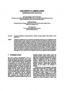
The document is then classified to that class j which returns the highest probability. In figure 8 we can see the performance of the Naive Bayes classifier. As can be seen, though the algorithm performs reasonably well when the number of labeled examples per class is close to 100, when the number of labeled examples is low, the algorithm fails to reach high performance. In each case the classifier is tested on the remaining examples. Thus when 100 labeled examples are used per class, then the resulting classifier is tested on the remaining 3930200=3730 examples. In order to obtain representative results, for each number of labeled examples per class, the experiments are repeated 10 times, each time the labeled examples being chosen by drawing with a uniform distribution without replacement from the set of 3930 examples. 0.95
0.9
Accuracy
0.85
0.8
0.75
0.7
0.65 Naive Bayes Classifier 0
20
40 60 80 Number of Labeled Examples per Class
100
Figure 8 As can be seen by the results obtained the Naive Bayes classifier performs quite well when the number of examples is sufficient, 20
reaching an accuracy of 90 percent when the number of labeled examples per class are 100, when the number of examples per class are few the accuracy of the classifier falls dramatically (as can be expected). This seems to be a first indication that document classification may very well benefit from transductive learning as at least this supervised algorithm performs unsatisfactorily for small amounts of labeled data. 2.3.2
SVM
Support Vector Machines have been used in a wide variety of applications and have been shown to attain high performance in most cases. They belong to a class of classifiers known as linear classifiers which aim to learn the solution to classification problems using a linear function. Specifically the aim of linear classification machines is given a set of examples (input) x = (x1 , x2 ...xn ) and a corresponding set of labels (output) y = (y1 , y2...yn ) where in the binary classification case yi ∈ {−1, 1}, to learn a function f (x) =< w · x > +b such that f (xi ) ≥ 0 if yi = 1 and f (xi ) < 0 if yi = −1. The problem however of finding a separating hyperplane such that instances belong to one class lay on ones side of the hyperplane and instances belonging to the other class lay on the opposite side, does not have a single solution. Thus if the data is linearly separable, then there are an infinite number of functions f (x) =< w · x > +b that given a set of examples and corresponding labels, satisfy the restrictions f (xi ) ≥ 0 if yi = 1 and f (xi ) < 0 if yi = −1 [4]. The simplest model of a support vector machine, works only for linearly separable data, is the so called maximal margin classifier. The margin of an example (xi , yi ) with respect to a hyperplane (w, b) is defined to be the quantity: γi = yi (< w · xi > +b) If γi > 0 then from the above equation it is evident that the example xi is classified correctly by the function f (x). By extension the margin distribution of a hyperplane (w, b) with respect to a training set S = ((xi , yi), ..., (xl , yl )) ⊆ (X × Y ) is the distribution of the examples in S. The minimum of the margin distribution (i.e. the minimum margin over all the examples of the set S) is the margin of the hyperplane (w, b) with respect to the training set S.
21
By normalizing the linear function we obtain the separating hy1 1 perplane ( kwk w, kwk b) and the corresponding geometric margin which is in fact the Euclidean distance of the points from the decision boundary in the input space [4]. The margin of a training set S is the maximum geometric margin over all hyperplanes and the corresponding hyperplane is the maximal margin hyperplane.
Figure 9 Thus a simple support vector machine solves the linear separation problem by finding a separating hyperplane such that the minimum geometric margin is maximal. This translates to the hyperplane whose distance from the closest points (to it) in the input space is as large as possible. By fixing the functional margin to one we can optimize the corresponding the geometric margin by minimizing the norm of the weight vector. This is evident if we consider the following. Let us suppose that the closest positive point to the hyperplane is x+ and the closest negative x− , this implies [4] : < w · x+ > +b = +1 and < w · x− > +b = −1
22
and the geometric margin is given by [4]: w w γ = 21 (< kwk · x+ > − < kwk · x− >) = 2 2 1 = 2kwk (< w · x+ > − < w · x− >) = 2 1 = kwk 2
Thus the problem can be transformed to the equivalent optimization problem: minimize < w · w > subject to yi (< w · xi > +b) ≥ 1 Unfortunately it is seldom the case that the examples of set S are linearly separable. In most cases it is not possible to find a hyperplane (w, b) such that the examples belonging to each class lay on opposite sides of the hyperplane. In order to overcome this problem and create a support vector machine that can solve the maximal margin classification problem even in the cases where the data is not linearly separable, we first introduce the notion of the margin slack variable of an example (xi , yi ) [4]. For a specific fixed value γ > 0 the margin slack variable ξi of an example (xi , yi) with respect to a hyperplane (w, b) and the target margin γ is defined as : ξi = max(0, γ − yi (< w, xi > +b)) This quantity can be seen as a measure of how much the specific point (xi ) fails to have a margin γ from the hyperplane (w, b). If ξ > γ then obviously xi is misclassified by the hyperplane (w, b). The norm kξk measures the amount by which the training set fails to have a margin of γ, taking into account any misclassifications that may appear in the training data.
23
Figure 10 With the help of the slack margin variable we can restate the optimization problem to allow for the margin constraints to be violated. This gives the so called soft margin optimization problem which is [4]: minimize < w · w > +C
l P
ξi
i=1
subject to yi (< w · xi > +b) ≥ 1 − ξi This is the 1-norm soft margin case which will be used throughout the experiments conducted here. In the 2-norm case the objective l P function to be minimized is : < w · w > +C ξi 2 . i=1
As stated above, a support vector machine (in the 1-norm soft margin case) ultimately solves the optimization problem. Programming SVM
minimize < w · w > +C
l P
ξi
i=1
subject to yi (< w · xi > +b) ≥ 1 − ξi The problem stated above is presented in the so called primal form. Before we continue to the actual programming of the support 24
vector machine we first transform the optimization problem to its dual form using Lagrange multipliers [4]. Thus the optimization problem becomes : maximize W (a) =
l P
i=1
ai −
subject
l P
1 2
l P
yi yj ai aj K(xi , xj )
i,j=1
yi ai = 0
i=1
and 0 ≤ ai ≤ C where K(x, z) is a kernel function which implicitly maps the input to a feature space. In the case where no kernel is used we have : K(x, z) =< x · z >. The bias b no longer appears in the dual form but is given by the equation [4]: b∗ = −
maxyi =−1 (w ∗ ·xi )+minyi =1 (w ∗ ·xi ) 2
P where w ∗ = yi a∗i xi is the solution to the optimization problem. Having converted the optimization problem to its dual form, we can proceed to programming the support vector machine. The simplest approach is to use gradient descent, meaning that the vector a is sequentially updated following the steepest ascent in the direction of the gradient of W (a). Using this method, the examples of the training set are sequentially presented to the support vector machine and the component ai is updated by the rule : ai = ai + ηi (1 − yi
l P
aj yj K(xi , xj ))
j=i
where ηi is the learning rate and can be proven to provide maximal gain for ηi = K(x1i ,xi ) . In order to satisfy the restrictions of the objective function, after each update we perform a check to make sure that the update ai is not below zero or above C, if this is the case then we set ai = 0 or ai = C accordingly. This approach however proves to be impractical as its complexity makes it excessively time consuming. Instead we program a support vector machine using the sequential minimal optimization (SMO) algorithm [15]. This algorithm is based on a technique known as decomposition in which only a subset of the Lagrange multipliers ai 25
are considered at each moment with the rest considered constant. In the case of the SMO algorithm this idea is taken to the extreme and only two multipliers are considered at a time. One of the main ideas is that in the case of only updating two multipliers at a time, there exists an analytical solution to the optimization problem. More analytically, considering a1 and a2 to be the multipliers to be updated, then the new values for these two parameters must lie l P on a line in order not to violate the linear conditions ai yi = 0. i=1
Thus we have :
old a1 y1 + a2 y2 = constant = aold 1 y1 + a2 y2
where of course the constraints 0 ≤ a1 , a2 ≤ C must also be satisfied. This translates to the following constraints for the value anew : 2 U ≤ anew ≤V 2 where old old old U = max(0, aold 2 − a1 ), V = min(C, C − a1 + a2 )
if y1 6= y2 , and old old old U = max(0, aold 1 + a2 − C), V = min(C, a1 + a2 )
if y1 = y2 . It can be proven [4] that the maximum of the objective function y2 (E1 −E2 ) can be achieved by first computing anew,unc = aold and 2 2 + κ clipping it to enforce the constraints U ≤ anew ≤ V . Where −κ = 2 −K(x1 , x1 ) − K(x2 , x2 ) + 2K(x1 , x2 ) is the second derivative of the objective function along the diagonal line and Ei = f (xi ) − yi = (
l P
j=1
aj yj K(xj , xi ) + b) − yi
is the difference between function output and target classification of the point xi . The value anew can then be obtained from anew as follows : 1 2 old new anew = aold 1 1 + y1 y2 (a2 − a2 ).
26
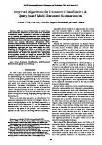
In figure 11 we can see the performance of the support vector machine. As before the experiments were repeated 10 times each time drawing the labeled examples from the dataset by using a uniform distribution without replacement. Once the SVM was trained using the examples, its performance was observed on the remaining examples in the data set. From the figure we can see that once again in the case of a supervised learning algorithm the problem cannot be solved to a satisfactory level when very few labeled examples exist. This reinforces the suspicion that when it comes to document classification, the problem cannot be solved satisfactorily with supervised algorithms if there is not adequate labeled data. SVM Results
0.95
0.9
Accuracy
0.85
0.8
0.75
0.7
0.65 Support Vector Machine 0
20
40 60 80 Number of Labeled Examples per Class
100
Figure 11 2.4 2.4.1
Transductive Learning Algorithms Self-Training
One of the simplest transductive learning algorithms, is the selftraining algorithm [12]. In self-training, a learner L is trained using the labeled examples of the training set. Once the learner has been trained, it is used to classify the unlabeled examples. The most 27
confidently classified examples are then chosen and are labeled accordingly. These labeled examples are then added to the training set and the learner is retrained. The process continues iteratively, each time the learner being trained with a slightly augmented training set. This can continue until every example in the original test set is labeled or (as this can prove to be especially time consuming) after a fixed number of steps. In the experiments conducted here, the learner used was a Naive Bayes Classifier. Thus after the training set has been used to obtain the parameters ϑcj = P (cj |ϑ) and ϑwt |cj = P (wt |cj ; ϑ) of the model, the self-training algorithm calculates the probabilities of each document di for each of the classes cj : ˆ = P (cj |di; ϑ)
ˆ (di |cj ;ϑ) ˆ P (cj |ϑ)P ˆ P (di |ϑ)
and for each of the classes cj find those documents di which have ˆ and labels them accordingly. the highest probability P (cj |di; ϑ) In the experiments conducted here, at each iteration of the algorithm, only the most confident example for each class is labeled, the process continues for 10 iterations, i.e. 10 examples are labeled for each class. Of course the process could continue until all the unlabeled examples are labeled (which translates to 3730/2 = 1865 iterations for the case of 100 labeled examples per class) but that proves impractical as the complexity of the Naive Bayes classifier makes it prohibitive. As in the cases before, the experiments are repeated 10 times and the resulting classifier tested on the unlabeled examples. The results of these experiments can be seen in figure 12. As can be seen the resulting classifier continues to perform badly for minimal labeled data (1 or 2 per class) but nonetheless performs quite well when the number of labeled examples are few (but not minimal). The sudden jump observed in the accuracy of the algorithm can be easily explained if one takes into consideration the nature of the algorithm. As at each iteration the algorithm augments its training set and retrains the classifier using the augmented training set, in order for its performance to increase the examples labeled must in fact belong to the class they are labeled to, otherwise they will hinder the training process. When the number of original labeled data is very small then the examples are labeled more or less randomly and 28
as the probability of the training set incorporating falsely labeled data increases, the accuracy of the algorithm instead of increasing with every iteration in fact deteriorates. When however the number of originally labeled examples surpasses a certain threshold then the examples chosen for labeling are highly likely to be classified correctly (as the original classifier is of a sufficient accuracy) and the algorithm no longer deteriorates but instead improves with each iteration. 0.95 0.9 0.85
Accuracy
0.8 0.75 0.7 0.65 0.6 SelfTraining 0.55
0
20
40 60 80 Number of Labeled Examples per Class
100
Figure 12 2.4.2
Transductive Expectation Maximization
A well known algorithm in statistical learning theory is the expectation maximization algorithm [14]. This algorithm uses iterative optimization in order to estimate some unknown parameters ϑ of a probabilistic model. In a supervised learning setting, expectation maximization is usually used when there is incomplete data present, i.e. the values of the different attributes are not all known for each example. Thus in these cases, expectation maximization is used to make a maximum likelihood estimation of the missing values. 29
In the case of transductive learning, the missing values are considered to be the labels of the unlabeled data. In particular, we consider a Bayesian probabilistic framework and originally train a Naive Bayes classifier using the labeled data. Having built the classifier using the labeled data, it is then used to estimate the component membership of each document. This translates to calculating the probability that each mixture component generated each document and based on these probabilistically weighted class labels are assigned to the unlabeled data. The algorithm then continues to train a new Naive Bayes classiˆ this time using the entire data set. The fier (i.e. new parameters ϑ) process of building classifiers and estimating labels for the unlabeled data is repeated iteratively until there is no change to the values of the estimated parameters ϑˆ (in practice the algorithm halts when the change in the log-likelihood of the data falls beneath some threshhold, in this case 10−4 ). Thus we effectively execute a hill-climbing search which ultimately calculates those labels for the unlabeled data that maximizes the value lc (ϑ |D) = log(P (ϑ)P (D |ϑ)) which is equivalently[14]: lc (ϑ |D; z) = log(P (ϑ)) +
|C| P P
di ∈D j=1
zij log(P (cj |ϑ) P (di |cj ; ϑ))
where zij are the indicator values of document di and where zij = 1 iff yi = cj , otherwise zij = 0. Consequently, the hill-climbing procedure effectively computes the expected value of z at each Estep and uses these values to estimate the maximum a posteriori ˆ As the labels estimates for the parameters of the mixture model ϑ. of the unlabeled data are not in fact binary, but rather, as stated, probabilistically weighted estimations of the true labels, when estimating the maximum a posteriori values for the parameters ϑˆ we use the following equations[14]: ˆ = ϑˆwt |cj = P (wt |cj ; ϑ)
1+ |V |+
|D| P
N (wt ,di )P (yi =cj |di )
i=1 |V P| |D| P
s=1 i=1
N (ws ,di )P (yi =cj |di )
where N(wt , di ) is the count of the number of times word wt appears in document di . The value P (yi = cj |di ) ∈ {0, 1} for labeled data, while in the case of labeled data we have P (yi = cj |di ) ∈ [0, 1]. The class prior probabilities are given by [14]: 30
ˆ = ϑˆcj = P (cj |ϑ)
1+
|D| P
i=1
P (yi =cj |di )
|C|+|D|
. The above equations are derived from the maximum a posteriori parameter estimation, if we consider the prior distribution over the parameters (P (ϑ)) to be a Dirichlet distribution[14]: Q Q P (ϑ) ∝ ((ϑcj )a−1 (ϑwt |cj )a−1 ) cj ∈C
wt ∈V
The parameter a affects the strength of the prior, if we consider a = 2 which is equivalent to Laplace smoothing, then we obtain the formulas shown above[14]. In figure 13 we can see the performance of the Expectation Maximization algorithm. As in the case of Selftraining, the experiments were repeated ten times each time drawing the labeled examples by a uniform distribution without replacement and the resulting classifier each time being tested on the remaining (originally) unlabeled examples. 0.9
0.85
Accuracy
0.8
0.75
0.7 Expectation Maximization 0.65
0
10
20
30 40 50 60 70 80 Number of Labeled Examples per Class
Figure 13
31
90
100
As can be seen from these results, the algorithm quickly reaches a high performance as the number of labeled examples rises. Unlike the self-training algorithm however, expectation maximization does not deteriorate for minimal amounts of labeled data. On the contrary it reaches a relatively high performance (≈ 68%) even when originally there is only one labeled example per class. This performance is higher than both the supervised algorithms and the self-training transductive algorithm. The expectation maximization transductive learning algorithm, after having trained the first learner, in all subsequent iterations and training of a new classifier (at the M-step), uses both the labeled ˆ and the (originally) unlabeled data to estimate the parameters ϑ. These two sets of data are taken into consideration with equal weight and influence any estimations made equally. However it is obvious that there should be more confidence in the label of the labeled data than the labeling of the unlabeled data. Thus it would be preferable if during the M-step of the algorithm, i.e. the training of the Naive Bayes Classifier, the labeled data was taken more into account than the unlabeled data, especially seeing as the unlabeled data is far larger in quantity than the labeled data and subsequently it is highly probable that the information provided by the labeled data be lost under the weight of the information provided by the unlabeled data. In order to overcome these problems, an extra parameter λi is introduced which weights the contribution of each example di to the learning process. By introducing this variable, the quantity which is maximized by the expectation maximization algorithm is[14]: lc (ϑ |D; z) = log(P (ϑ)) + λ(
|C| P P
di ∈D u j=1
|C| P P
di ∈D l j=1
zij log(P (cj |ϑ) P (di |cj ; ϑ)) +
zij log(P (cj |ϑ) P (di |cj ; ϑ)))
where D u and D l are the sets of labeled and unlabeled documents. As λ approaches zero, the influence of the unlabeled data on the learning diminishes, the algorithm effectively reverts to supervised learning for λ = 0, while for λ = 1 the algorithm takes both labeled and unlabeled data into equal consideration. For the training process realised in the M-step, we define Λ(i) to be[14]: 32
Λ(i) = λ if di ∈ D u and Λ(i) = 1 if di ∈ D l Using these values, the formulas for computing the parameters ϑˆ become[14]: ˆ = ϑˆwt |cj = P (wt|cj ; ϑ)
1+ |V |+
|D| P
Λ(i)N (wt ,di )P (yi =cj |di )
i=1 |V P P| |D|
s=1 i=1
Λ(i)N (ws ,di )P (yi =cj |di )
and the class prior probabilities are given by : ˆ = ϑˆcj = P (cj |ϑ)
1+
|D| P
i=1
Λ(i)P (yi =cj |di )
|C|+|D l |+λ|D u |
In figure 14 we see the performance of the algorithm for different values of lambda. The settings of the experiments remain the same as before 0.95 0.9 0.85
Accuracy
0.8 0.75 0.7 0.65 lambda=1
0.6
lambda=0.5 lambda=0.2
0.55
lambda=0.1 0.5
0
10
20
30 40 50 60 70 80 Number of Labeled Examples per Class
Figure 14
33
90
100
From the results it can be seen that the introduction of the parameter λ does in fact improve the performance of the algorithm. However this improvement exhibits itself mostly when the number of labeled examples is not minimal. Thus for minimal amounts of labeled data, the algorithm performs best for λ = 1 which is equivalent to the original algorithm. The introduction of the parameter λ only leads to improvement as the number of labeled examples augments leading to a clear advantage when the number of labeled examples is above 20 per class. This makes sense if ones considers that for minimal amounts of labeled data, the information received by these examples is also minimal and thus the algorithm must rely on the unlabeled data. As however the number of labeled examples increases, the information for the labeled data also increases and so not only decreases the need for information from the unlabeled examples, but also so increases the need to protect this information from being buried under the unlabeled data’s information. 2.4.3
Transductive Learning Using Graph Mincuts
Another approach to transductive learning is that of using graph mincuts [1]. One of the main advantages of the graph mincut algorithm is that unlike the expectation maximization algorithm presented in the previous chapter, the graph mincut finds the global maximum of the objective function. Furthermore this global maximum can be found in polynomial time. However, while in the case of the expectation maximization algorithm, the hill-climbing procedure can be applied to a wide number of objective functions, in the case of the graph mincuts algorithm the objective functions are limited to those functions which depend only on pairwise relations amongst examples. In particular, the graph mincuts algorithm can perform the following optimization which is of great interest[1]: Given a set of labeled examples (in this case documents) D l and a set of unlabeled examples D u , label the unlabeled examples in such a way that the leave one out cross validation error of the k-nearest neighbor algorithm is minimized over the entire data set D = Dl ∪ Du.
Given these two sets of data D u and D l , the algorithm first constructs a weighted graph G = (V, E), where the vertices V consist 34
of one vertice for each example in the labeled and unlabeled data set and also a source vertix u+ and sink vertix u− ; thus we have V = D l ∪ D u ∪ {u+ , u− }. The vertices u+ and u− are also called classification vertices, while the other vertices are called example vertices. Each edge e ∈ E between the vertices in the graph is assigned a weight w(e). This weight can be assigned by any number of functions (for example analogously to the distance between the two examples that the edge connects), in the experiments conducted here the value of w(e) for edges e between two example vertices ui and uj is set to be w(e) =
cos(d~i ,d~j ) P cos(d~i ,d~m )
if example dj is amongst the k nearest
m∈kNN(di )
neighbors of example di (or vice versa), where cos(d~i , d~j ) is the cosine similarity function between documents di and dj and which is equal to : cos (d~i, d~j ) =
d~i ·d~j ~ kdi k2 ∗kd~j k2
=
s
n P
k=0 n P
k=0
wik wjk s n P 2
wik
k=0
2 wjk
Otherwise if dj is not amongst the nearest neighbors of di then the weight of the edge between the two vertices is set to 0, i.e. the vertices are not considered to be connected. In the case of the classification vertices u+ and u− , these are connected to those vertices which correspond to labeled data with the same label as the corresponding classification vertex. Thus vertices corresponding to positively labeled examples (i.e. examples with a label of +1) are all connected to the vertex u+ , while vertices corresponding to negatively labeled examples (i.e. examples with a label of -1) are all connected to the vertex u− . These edges between classification vertices and example vertices are all assigned an infinite weight, thus we have w(u, u−) = ∞ xor w(u, u+) = ∞ ∀u ∈ D l . The algorithm then proceeds to calculate a minimum cut for the graph, considering u+ as the source and u− as the sink which translates to finding the minimum total weight set of edges that disconnect u+ and u− . This can be achieved with the help of a maximum flow algorithm like for example the Edmonds-Karp algorithm [2] which is used in the following experiments. Before analyzing in detail the Edmonds-Karp algorithm, we must first introduce the notion of the residual network. Given a graph 35
G = (V, E) with capacity c(v, u) and flow f (v, u) between vertices v and u, the residual network Gf (V, Ef ) is the network with capacity cf (v, u) = c(v, u) − f (v, u). The Edmonds-Karp algorithm is based on the Ford-Fulkerson algorithm [2] which uses the residual network to solve the maximum flow problem of a graph, as follows :
While there is a path p in Gf from s (source) to t (sink) such that cf (u, v) > 0 ∀(u, v) ∈ p then : Set cf (p) = min(cf (u, v)|(u, v) ∈ p). ∀(u, v) ∈ p do : f (u, v) = f (u, v) + cf (p) f (v, u) = f (v, u) − cf (p) The Edmonds-Karp algorithm is a variation of the Ford-Fulkerson algorithm which specifically uses depth-first search to find the path p in the residual network Gf . Returning to the transductive learning graph mincut algorithm, having found the mincut of the constructed graph, the graph is essentially partitioned into two sets V+ and V− each consisting of vertices situated on opposite sides of the mincut. Thus vertices in V+ are those vertices which can be reached by a path p in the final residual graph and which form a connected component which includes the vertex u+ while conversely vertices in the set V− cannot be reached by a path p in the final residual graph. Finally the unlabeled examples corresponding to the vertices in each of the two subsets are labeled accordingly. Figure 15 shows the performance of the graph mincut algorithm for various quantities of labeled examples. As before, the experiments are repeated 10 times, each time the labeled examples being drawn from the extended data set using a uniform distribution without replacement. The graph was constructed considering the 3-nearest neighbors of each example [1].
36
0.95 0.9 0.85
Accuracy
0.8 0.75 0.7 0.65 0.6 MinCut 0.55
0
20
40 60 80 Number of Labeled Examples per Class
100
Figure 15 The results obtained using the graph mincut transductive learner show that once again the transductive learning algorithm is able to reach relatively high levels of performance with a few labeled examples per class. However unlike the expectation maximization algorithm in the previous section, the algorithm is unable to attain a high performance when the number of labeled examples is minimal. In fact in the case of one labeled example per class the algorithm performs worse than the supervised algorithms, its performance bordering on that of a random classifier. A possible explanation for this phenomenon is presented in the next section along with an alternative graph partitioning algorithm which aims to remedy this problem. 2.4.4
Tranductive Spectral Graph Partitioning
The graph mincut algorithm presented in the previous chapter is a intuitively appealing approach to the transductive learning problem, however it does not in all cases lead to similarly appealing solutions. Consider the case where there are only two labeled examples, one 37
positive x+ and one negative x− . If we connect each point to its three closest neighbors then it is very likely that the minimum cut of the graph consists of partitioning the graph into two sets S and S¯ such that S = u+ ∪, x+ and S¯ = u− ∪ x− ∪ D u . This partition obviously will result in every example in the unlabeled data set D u being labeled with a negative label. In this case it is obvious that the resulting classifier performs substantially poorer than if we had not taken the unlabeled data into consideration at all. The problem of degenerated cuts can be overcome if we consider the graph Laplacian and instead of the minimum cut problem, we solve the ratiocut problem instead [8]. The ratio of a cut S, S¯ is defined as : ¯ = R(S, S)
¯ S) P C(S,P di di ·
i∈S
i∈¯ (S)
¯ is the sum of the where di is the size of vertex i and C(S, S) ¯ The ratio weights of the edges between the vertices of S and S. cut problem consists of finding the non-empty cut S, S¯ for which ¯ is minimum. Thus instead of minimizing the sum the value R(S, S) of the weights of the edges of the cut as in the case of the mincut problem, the ratiocut problem finds the cut S, S¯ which minimizes the average weight of the cut. The Laplacian LG of a graph G = (V, E) is a matrix whose entries lij are given by : lij = −1 if (i, j) ∈ E lij = di if i = j where di is the degree of vertex i lij = 0 otherwise. The Laplacian of a graph provides information about various characteristics of the graph through its eigenvalues λi and corresponding eigenvectors vi . For example the multiplicity of 0 as an eigenvalue of LG equals the number of connected components of G. In the case of the ratiocut problem, the eigenvalue λ2 (i.e. the smallest non-negative eigenvalue) is important as it yields information concerning the quality of the best cut of the graph. ¯ to be : If we redefine the ratio of a cut (S, S) φ(S) =
¯ | |C(S,S) ¯ | min(|S|,|S)
38
then the isoperimetric number φ(G) of a graph can be defined as : φ(G) = minS φ(S) It is obvious from the above that the ratiocut problem consists of finding a cut in the graph whose ratio is equal to the isoperimetric number. The isoperimetric number is related to the eigenvalue λ2 via Cheeger’s inequality : φ(G) ≥ λ2 ≥
φ2 (G) 2d
where d is an upper bound of the degree of every vertex in the graph. Thus the eigenvalue λ2 of the Laplacian LG bounds the isoperimetric number of the graph, giving both a lower bound (φ(G) ≥ λ2 ) and a √ higher bound ( 2d · λ2 ≥ φ(G)). Before presenting the spectral graph transducer [8] that solves the spectral graph partitioning problem in a transductive setting, we first formally state the problem to be solved. Given a graph G = ¯ C(S,S) (V, E) the problem consists of minimizing the value |i:yi =1||i:y i =−1| l with the constraints a) yi = 1 if i ∈ D and positive, b) yi = −1 if i ∈ D l and negative and c) ~y ∈ {+1, −1}n . Ignoring these constraints which are related to the labels of the labeled data set, we obtain the unsupervised ratiocut problem which is equivalent to the following[8]: T
z min~z ~z~zTL~ ~ z q q |i:zi >0| i 0| − |i:zi d − < vi , hj >c +cost ∗ wij ) The value of < vi , hj >d is the fraction of times the units i and j, in the input and output layer respectively, are both ”on” when the input of the machine is an example of the data set; the value of < vi , hj >c is accordingly the fraction of times the units i and j, in the input and output layer respectively, are both ”on” when the input of the machine is a confabulation. At each update k, the value of the previous update k − 1 is also taken into account via the term m ∗ ∆wij k−1. Furthermore the value of the weight itself is also taken into consideration via the term cost ∗ wij . As can be seen by the update rule given, the training process aims to minimize the energy over the data while raising the energy of the confabulated data. Once the restricted Boltzmann machine is trained, the process of pretraining weights continues to the next pair of network layers where obviously the new input layer is the previous output layer. Having pretrained the network and obtained weights that hopefully are more suitable, the network can then be trained. In the case of the pretrained network presented here, the network is subsequently trained using a conjugate gradient method [18]. In the conjugate gradient method the search for the (local) minima of the function is conducted in directions that are A-orthogonal. 61
Two vectors are A-orthogonal (or conjugate) if the following equation holds : di T ∗ A ∗ dj = 0 Choosing the search directions to be A-orthogonal guarantees the method will find the (local) minima after at most n steps, where n is the dimensionality of the search space. As is known the minimization of a quadratic function f (x) requires the determination of a set of values for which f ′ (x) = 0. These values are determined by the solution of an equation of the form: Ax = b In each of the A-orthogonal directions di−1 a search is conducted to find the value xi for which the error vector ei = Axi − b is Aorthogonal to di−1 . The directions chosen for search are given by the following iterative equations: di+1 = ri+1 + βi+1 di r T ri βi = rT i ri−1 i−1 and ri = −Aei Where the vectors ri are the residuals. For these residuals we have also that ri = b − Axi . In the case of nonlinear problems these vectors are in fact the directions of steepest descent. In the experiments conducted for the conjugate gradient finetuning, Carl Rasmussen’s minimize code was used .Batch training was implemented in the fine-tuning stage and for each epoch and for each batch presented for training, three line searches were conducted. The restricted Boltzmann machines were each trained for 50 epochs with a learning rate of 0.1, a cost weight of 0.0002, the parameter m was set to 0.5 for the first five epochs and 0.9 for all subsequent. The experiments were repeated ten times, each time drawing the labeled examples from the data set using a uniform distribution without replacement and the trained network tested on the remaining unlabeled examples. The results of these experiments can be seen in figure 25.
62
0.75 0.7 0.65
Accuracy
0.6 0.55 0.5 0.45 0.4 Pretrained Network (RBM) 0.35
0
5 10 Number of Examples per Class
15
Figure 25 The results show that the pretrained network ,unlike the convolutional networks, are in fact able to learn from such small amounts of data. However the results are far from satisfactory, it is characteristic that for one or two labeled examples per class the network has an accuracy of below 50% and though this is much better than random (which would be 10%) it still means that the resulting classifier is wrong more times that it is right. 3.4 3.4.1
Transductive Learning Expectation Maximization
In the case of transductive learning using expectation maximization, when applied to handwritten digit recognition, we can no longer use a naive Bayes classifier as a base learner. A naive Bayes classifier (based on a multinomial model) considers each example to be an ordered series of events. This approach does not seem appropriate when it comes to images, as in this case the classifier would consider a pixel of intensity 255 (for example) to be the result of a specific event (corresponding to specific pixel) occurring 255 times, which 63
would seem to make little sense. Thus rather then use a naive Bayes classifier as a base learner, we must turn towards other solutions. An alternate framework that would seem to be well suited for the transductive expectation maximization is that of considering the data as generated by a mixture of normal (Gaussian) densities[5]: p(x) =
c P
i=1
1
T Σ−1 (x−µ ) i i
1 − 2 (x−µi ) P (ωi) √2π|Σ| 1/2 e
where AT is the transpose of A. The probabilities P (ωi) are the prior probabilities of each class ωi , while the values µi and Σi are the mean and covariance matrix respectively that correspond to class ωi . Based on the above assumption given a specific example xk , the probability P (ωi |xk ) is given by[5]: P (ωi|xk ) =
Pp(xk |ωi )P (ωi ) p(xk |ωj )P (ωj ) j
and the most probable class for the example xk is given by[5]: k |ωi )P (ωi ) ω(xk ) = argmaxi P (ωi |xk ) = argmaxi Pp(x p(xk |ωj )P (ωj ) j
As the denominator
P j
p(xk |ωj )P (ωj ) is common for all P (ωi|xk )
it can be ignored and thus the above equation becomes: ω(xk ) = argmaxi p(xk |ωi )P (ωi) and substituting p(xk |ωi ) = the final form :
√
1 − 12 (x−µi )T Σ−1 i (x−µi ) 1/2 e 2π|Σ|
1
we obtain
T Σ−1 (x−µ ) i i
1 − 2 (x−µi ) P (ωi |xk ) = P (ωi) √2π|Σ| 1/2 e
In the above final equation, the mean of each class ωi is the expected value of an example generated by the mixture component corresponding to that class µi = E[x]. Given a data set D, if the maximum-likelihood estimates are used then the mean of each class ωi is given by[5]: µi =
1 n
n P
k=1
64
xk
where obviously, xk is considered to belong to class ωi . Equivalently the maximum-likelihood estimate of the covariance matrix Σi of class ωi is given by[5]: Σi =
1 n
n P
(xk − µi )T (xk − µi )
k=1
where as above xk is considered to belong to class ωi . Finally the probabilities P (ωi ) are given by [5]: P (ωi) =
n N
where n is the number of examples in the data set belonging to class ωi and N is the size of the data set. Based on the above we can use this framework for transductive learning with the help of the expectation maximization algorithm. At each E-step of the algorithm the parameters µi ,P (ωi) and Σi are calculated for each class ωi using the data. In the first E-step only the labeled data is used while in subsequent steps the extended data set is used as after the first M-step all the examples are assigned a label. Subsequently in the M-step, the probabilities p(xk |ωi ) are calculated ∀k, i and each example xk is assigned a label accordingly. Unfortunately even though the presented framework ties in naturally with the expectation maximization algorithm, in the case of the experiments presented here it cannot be applied due to a number of problems that arise and make the algorithm in its present form inapplicable. In particular, the experiments conducted here focus on the case where there are very small amounts of labeled data. These settings are natural when conducting experiments on transductive learning as when large amounts of labeled data are present, supervised methods are more appropriate. This scarcity of labeled data however means that though it is possible to calculate the maximum-likelihood estimates of the covariance matrices Σi , these estimates will not be inversible. This is due to the fact that in order for the covariance matrix Σi = n P 1 (xk − µi )T (xk − µi ) to be inversible the number of examples n n k=1
must be at least as large as the dimensionality of the data d. As the data has 784 dimensions and the labeled data sets used here are
65
of a size of maximum 15 examples per class, it is evident that the resulting matrices will not be inversible. One way to overcome this problem is to assume that every class has the same covariance matrix Σ. The entire data set (both labeled and unlabeled data) can then be used to calculate this covariance matrix and since the size of the data set N is 4000 examples it is obvious that N ≥ D. Thus we have : Σ=
1 n
N P
(xk − µi )T (xk − µi )
k=1
Unfortunately, though this approach overcomes the initial approach of insufficient labeled data, it suffers from a further setback. As stated the data consists of images of digits which have been centered on a 28 × 28 background. This means that the pixels near the border of the image tend to have a value of zero, as the pixels of the digit tend to be more towards the center. In fact there are lines of pixels whose value is constantly zero over the entire data set. This unfortunately means that the respective rows in the covariance matrix Σ are also zero which in turn means that rank(Σ) < d. Thus once again the covariance matrix is not inversible. In order to overcome this obstacle, we employ two different approaches that ultimately prove successful. The first approach is to use a technique known as shrinkage which ”‘shrinks”’ the covariance matrix Σ towards the identity matrix I[5]: Σβ = (1 − β)Σ + βI The results of experiments conducted using this approach can be seen in figure 26 where the accuracies for different numbers of labeled examples per class in relation to the number of steps of the expectation maximization algorithm are shown. The settings of the experimentation (creation of training set, test set and repetitions) remain the same as in the supervised experiments. The parameter β is set experimentally to 0.8.
66
0.75 0.7 0.65
Accuracy
0.6 0.55 0.5 1 Example per Class 2 EpC 5 EpC 8 EpC 12 EpC 15 EpC
0.45 0.4 0.35
1
1.5
2
2.5
3 Steps
3.5
4
4.5
5
Figure 26 As can be seen in almost every case, after one or at the most two iterations of the algorithm, the performance of algorithm ceases to improve and from then on any further iterations are counterproductive. If we chose to run only two iterations (which seems to be the optimal) then the performance of the algorithm can be seen in figure 27.
67
0.75
0.7
Accuracy
0.65
0.6
0.55
0.5
0.45
0
5 10 Number of Examples per Class
15
Figure 27 It is evident from the results obtained that though the selftraining algorithm may perform better than the supervised pretrained networks, they nonetheless do not seem to completely overcome the problem of poor performance for small amounts of labeled data. Thus in this case the presence of unlabeled data may lead to an improved performance, however this performance is still relatively low. The second approach to calculating an inversible covariance matrix is to assume that the features are statistically independent and that each of the features has the same variance σ 2 . This leads to a common covariance matrix of the form[5]: Σ = σ2 I which is obviously inversible. In order to calculate the variance σ 2 , an average of the variance over the data set of each feature is calculated. The results obtained using this approach can be seen in figure 28 for various numbers of iterations of the algorithm.
68
0.75
0.7
Accuracy
0.65
0.6
0.55
0.5
0.45
0.4
1
1.5
2
2.5
3 Steps
3.5
1 Example per Class 2 EpC 5 EpC 8 EpC 12 EpC 15 EpC 4 4.5 5
Figure 28 As can be seen with the exception of the cases where only one or two examples per class are labeled, the algorithm does not gain in performance from using expectation maximization. Thus in order to use the expectation maximization algorithm we must revert back to the previous approach. 3.4.2
Self-Learning
As was the case with the transductive learning algorithm using expectation maximization, in the case of self-learning once again a naive Bayes classifier is not a suitable base learner for the same reasons as above. Instead of using a naive Bayes classifier, again as before we assume that the data has been generated by a mixture of Gaussian distributions. The self-training algorithm in this case, calculates the covariance matrix Σ (using the approaches described) the means of the classes µi and the prior probabilities P (ωi), the latter two using the labeled data while the former using the entire data set. The algorithm then calculates the probabilities P (ωi |xk ) and for 69
each class ωi labels the example xk for which the value P (ωi|xk ) is maximal over the data set. The algorithm then continues to iteratively calculate parameters and label examples, extending the labeled data set each time by one example per class. Unfortunately as can be seen from figure 29, in the case of self-training the results obtained show that the performance of the learner does not improve. The results are obtained using the standard experimentation settings used in the previous sections. 0.8
0.7
Accuracy
0.6
0.5
0.4 1 Example per Class 2 EpC 5 EpC 8 EpC 12 EpC 15 EpC
0.3
0.2
0.1
1
2
3
4
5
6
7
8
Steps
Figure 29 As the framework used with the expectation maximization algorithm does not seem to work in the case of self-learning, we must choose a different learner as a base, in order to obtain a self-learning transductive classifier with enhanced performance. For this purpose we experiment with using a class of neural networks known as autoencoders [7]. Autoencoders are typically used to reduce the dimensionality of the data. The main architectural idea behind these networks is a bottlenecked network which has as many output neurons as input and has a hidden layer with as many neurons as the desired 70
dimensionality of the data (obviously less than the original dimensionality). By equating the target of the network with the input presented each time we force the bottlenecked hidden layer to learn a representation of the data. As the autoencoding network is trained to replicate its input in its output layer, this means that the values of the neurons of the bottlenecked hidden layer hold adequate information so as to allow for the (optimally perfect) reconstruction of the input by the succeeding part of the network. In figure 30 the architecture of such an autoencoder can be seen.
Figure 30 In the experiments conducted here we use a series of autoencoding networks in a slightly different fashion. Instead of aiming to reduce the dimensionality of the data, we use a number of autoencoders (as many as the different classes in the data) to create a classifier. Each of the autoencoders is trained using only that data which belongs to a specific class. This way, each autoencoder is trained to replicate only those examples that belong to its specific class. The unlabeled data is then passed through each of the autoencoding networks and each example is classified according to which autoencoder best replicates the example in its output. As in the case of the supervised pretrained network, the weights of the autoencoding networks are pretrained before the actual training phase. The weights between layers up until the bottlenecked layer 71
are as before considered to belong to a restricted Boltzmann machine whose input layer consists of linear units with Gaussian noise and whose hidden layer consists of units with binary states. The training process of this RBM is very similar to the process in the supervised case. For each example presented to its input, the RBM calculates the probabilities of the output units hj being ”‘on”’ [6]: P (hj = 1) = 1+e
1P
−bj −
i
vi ∗wij
As before, based on these values, a confabulation is also calculated : vi = 1+e
1P
−bj −
j
hj wij
and subsequently probabilities P (hj = 1) are calculated anew. After all the appropriate examples have been presented to the RBM, its weights are updated. The update rule used for the weights (for the kth update) is : ∆wij k = m ∗ ∆wij k−1 + lr ∗ (< vi , hj >d − < vi , hj >c +cost ∗ wij ) where at each update k, the value of the previous update k − 1 is also taken into account via the term m ∗ ∆wij k−1 . Furthermore the value of the weight itself is also taken into consideration via the term cost ∗ wij ). The terms < vi , hj >d and < vi , hj >c are as before the fraction of times the units i and j, in the input and output layer respectively, are both ”on” when the input of the machine is an example from the data set or a confabulation accordingly. The values of these terms are given by : P < vi , hj >= N1 vit ∗ Pt (hj = 1) t
where vit is the value of unit vi when the RBM is presented with the example (or confabulation) t. In the case of the bottlenecked layer, the RBM which has the units of this layer as an output is considered to have an output layer consisting of linear units. For each of these units, given a state of the input units v, the mean µj of the output unit hj is calculated 72
µj = bj +
P i
wij ∗ vi
The variance for each output unit is considered to be the same and equal to : σ 2 = 1. Having calculated the corresponding means, the machine then calculates the values of the output units by drawing from a normal distribution N(µj , σ 2 ). Based on these values, as before, a series of confabulations is calculated along with the corresponding values of the output units for those confabulations. Finally the weights are updated using the same update rule as before, only that in this case, the values of the terms < vi , hj >d and < vi , hj >c are given by : P < vi , hj >recon = N1 vit ∗ hj t
The process of pretraining the weights of the autoencoder is conducted up until the weights prior to the bottlenecked layer. The weights of the subsequent layers are obtained by ”unrolling” the network. Thus the weights between two layers situated after the bottlenecked layer are assigned the same values as the weights between the two corresponding layers prior to the bottleneck. This process of ”unrolling” can be seen in figure 31.
Figure 31 73
Subsequently the autoencoder is trained using the labeled examples as both input and target values. As before the method used during the training phase is the conjugate gradient method. After the ten autoencoders have been trained, the unlabeled examples of the data set are presented to each of these autoencoders. For each example xk and for each autoencoder i the reconstruction error Ei (xk ) is calculated. If oi is the output of autoencoder i, then the reconstruction error is given by: Ei (xk ) = koi − xk k2 Having passed through the entire set of unlabeled data, for each class i the unlabeled example xk for which Ei (xk ) is minimal over all the unlabeled data set is found and appropriately labeled, thus extending the labeled data set by one example per class. In figure 32 we can see the performance of the self-training algorithm based on autoencoders for various numbers of iterations. 0.8
0.75
Accuracy
0.7
0.65
0.6
0.55
2 Examples per Class 5 Epc 8 Epc 11 EpC 15 Epc
0.5
0.45
1
2
3
4
5
6
7
8
Steps
Figure 32 From figure 32 we can see that the performance of the algorithm seems to decline after a certain number of iterations, especially as the number of labeled examples per class rises. By fixing the number of iterations to three which seems according to the previous results to be the optimal, we obtain the results shown in figure 33, where the usual settings are used. 74
0.8
Accuracy
0.75
0.7
0.65
0.6
0.55
2
4
6 8 10 Number of Examples per Class
12
14
Figure 33 As can be seen by the results, the expectation maximization algorithm using autoencoders does not completely overcome the problem of low amounts of labeled data, as we shall see this transductive algorithm surpasses the supervised pretrained network algorithms in performance but as is evident from the results seen in figure 33, its performance is still not high. 3.4.3
A Convolutional Network Analogous
As can be seen by the results of the experiments conducted using convolutional networks, this supervised approach is not suitable when the number of labeled examples is very low. This inappropriateness can be readily explained if we consider the size of the convolutional network and the number of trainable parameters it has. Networks of this size typically require thousands of examples in order to be trained so it is not surprising that training fails when only a handful of labeled examples are available. Despite the extremely poor performance of convolutional networks in these settings, we can use the ideas it is based on (feature mapping and sub-sampling) to come up with a transductive learner which employs these two techniques with the help of the large quantities of unlabeled data to obtain a new representation of the data which allows for higher performance. As such the algorithms pre75
sented in this chapter are not classifiers themselves but rather a transductive method of acquiring a new data representation that can subsequently be combined with a classifier which will attain a higher performance. In order to create a feature mapping of the data that can exploit the available unlabeled data, we create feature detectors that can manipulate this data. To this extent we utilize a self organizing map (SOM) that will be trained to recognize the presence of certain features and thus serve as a group of feature detectors. This self organizing map takes a small number of input units which are situated in a small neighborhood of the data point (i.e. the SOM’s receptive field), and reveals in its output which feature is present in that neighborhood according to which of the SOM’s units is activated by the input. The SOM is originally trained using as input neighborhoods of units in the training data. Thus in the case where the SOM has a 5 × 5 input layer (as will be used here) the data used to train the SOM are 5 × 5 neighborhoods of input units taken from the original training data. By presenting the SOM with receptive fields taken from the data, it is trained to recognize a number of different features that are present in these 5 × 5 windows. Thus each neuron in the SOM’s output layer becomes sensitive to a different feature. Having trained the SOM, we subsequently scan each data point using this SOM in order to obtain a feature mapping of the data. For each data point the SOM is applied to consecutive receptive fields on the data point. Each of these receptive fields is shifted slightly in relation to the previous receptive field. Thus two consecutive receptive fields are overlapping as can be seen in Figure 34. Feature Mapping
76
Figure 34 By scanning each data point with the SOM, a feature mapping of the data point is created by recording for each receptive field which neuron in the SOM’s output field is activated. Thus the feature mapping of the data consists of a list of numbers as can be seen in Figure 35 where each of these numbers corresponds to a specific neuron in the SOM’s output field and denotes the presence of a specific feature in the corresponding receptive field. 1
4
7
5 8
9 9
1 3
12 11 9 4 10 8 5 4 1
3
5
6
1
7 1 11 7
3 2
12 1
10 11 4 1 12 1 3 1 2
7 7 5
1 2 11 4 7 1
5 1 9
1
9
1
2
1
4
5 1
1 9 11 5
1 4
1
1
4
8
1 9 1
7
9 3 3 1 10 4 1 3
12 1 1 7
3 9
2 1
7 3
4 1
3
9
11 5
7
2
1
Figure 35 Once a feature map of the data has been created, it is useful to find a way to execute sub-sampling. By using subsampling the algorithm will become even less sensitive to small disSub-Sampling
77
tortions in the data as the exact positions of the occurring features will no longer be as important as their approximate positions. To this effect, after creating the feature maps of the data, these feature maps are clustered in K different clusters. For each one of these clusters k we follow the following procedure : 1. A specific region (neighborhood) of units is extracted from the data points belonging to that cluster (here 2 × 2 neighborhoods are chosen). 2. The center of the cluster formed by these subdimensions is calculated. This center is treated as an archetype for that subregion in the specific cluster k 3. The above steps 1-2 are repeated scanning all the subdimensions of the data points. The subregions are chosen in such a way that they do not overlap. By this repetition we obtain a series of archetypal subregions for the entire data vector. 4. Steps 1-3 are repeated for all the clusters k. 5. Finally for each example in the data set, we compare each of its 2 × 2 subregions with the respective archetypes obtained for each of the clusters. The subregions of the data are then replaced with the archetype with which it has the greatest similarity. After this procedure has been executed the subdimensions of each data point consist of a series of archetypal subregions. Thus slight shifts or distortions in the original feature maps are lost as subregions exhibiting similar features will most likely be clustered together, and ultimately be replaced by a common archetype. Once a feature mapping of the data has been created and sub-sampling has been executed, the data acquires a new form of representation. However as the data is represented by a list of numbers denoting the presence of features and their locations, the Euclidean distance function is no longer an appropriate distance measure between two points. Instead the distance between two examples is calculated using a distance function based on the distances between neurons in the SOM’s output layer. Distance between Examples
78
More specifically the distance between two data points Ii and Ij is set to be the sum of the distances between the neurons in the SOM, for each pair of neurons activated by the same receptive fields in the SOM. More formally the distance between these two data points is calculated as dist(Ii , Ij ) =
M P
dSOM (Ii (k), Ij (k))
k=1
where Ii (k), Ij (k) denote the neurons activated by the k th receptive field of the two data points and where the distance function dSOM (x, y) returns the distance between neurons x and j in the self organizing map. Results using these methods can be seen in the following sections where the convolutional network analogous is combined with other transductive methods to form improved transductive classifiers. 3.4.4
Spectral Graph Partitioning
As analyzed in the previous chapter, the spectral graph transducer calculates the cut of a graph such that the average weight of the cut is minimal. Having found this cut, the algorithm labels the examples corresponding to nodes on the one side of the cut as positive and the examples corresponding to the rest of the nodes as negative. As such the spectral graph transducer is appropriate for binary classification problems. In the case however of the MNIST data set for handwritten digit recognition, the problem at hand is a multiclass one. Thus in order to be able to apply the spectral graph transducer to the handwritten digit recognition problem, it must first be altered in order to be able to handle multilabel problems. This adaptation is achieved by reconstructing the problem from a single multiclass problem to a series of binary classification problems. Thus in the case of c classes, we construct as many spectral graph transducers and train them using a one against all approach, for example the first spectral graph transducer is trained to discern between the digit 1 and the rest; in this case the examples of class ”-” are considered to be 1s while the examples in class ”+” are considered to be one (any) of the other digits. In this case the adjacency matrix is constructed based on the Euclidean distance of the examples,]. 79
The results when using the original representation of the data can be seen in figure 36 using the usual settings. We set c = 3200 and the adjacency matrix is constructed using the 5 nearest neighbours of each example. 0.8
0.75
Accuracy
0.7
0.65
0.6
0.55
0.5 SGT 0.45
0
5 10 Number of Examples per Class
15
Figure 36 Besides however applying the spectral graph transducer on the data using the original representation, the convolutional analogous presented in the previous chapter can also be used to obtain a new representation of the data. The adjacency matrix of the data is then constructed using the distance function analyzed in the previous chapter. Figure 37 shows the result of applying the transductive learner on the data when only feature mapping has been applied and when both feature mapping and sub-sampling have been applied; the previous results on the original representation are also shown for comparison. In the case where only feature mapping is applied, the experiments are repeated 25 times, 5 different self-organizing maps are trained using the data and for each of these SOMs we obtain a different representation of the data, for each of these representations we calculate an adjacency matrix for the data and repeat 5 experiments with the spectral graph transducer. In the case of both applying both feature mapping and subsampling, for each of the five representations (from the five different 80
SOMs) we cluster the data four times each time receiving a new sub-sampled representation. Thus we effectively obtain 20 different representations of the data. For each of these representations we repeat the experiment five times, effectively running 100 experiments for each amount of labeled data. 0.8
0.75
Accuracy
0.7
0.65
0.6
0.55 Original Representation Feature Mapping Feature Mapping + Sub−Sampling
0.5
0.45
0
5 10 Number of Examples per Class
15
Figure 37 As can be seen from the results above, applying feature mapping to the data prior to executing the spectral graph partitioning leads to an increase of the performance of the resulting classifier. Furthermore if sub-sampling is applied subsequent to the feature mapping and then the algorithm executed, the performance improves even further. Based on these results we can see that the convolutional analogous proposed does in fact contribute to the learning process. 3.4.5
Learning with Local and Global Consistency
In the case of transductive learning with local and global consistency, the application of the algorithm to the handwritten digit recognition problem is straightforward. As the algorithm is already adapted to handle multiclass problems, no alterations to the algorithm is needed. The only difference with the algorithm applied to the document classification problem is that the construction of the affinity matrix is slightly changed to better represent the nature of the problem. 81
The values of the affinity matrix W are given by : 2
Wij = e−kxi −xj k
/2σ2
when i 6= j and Wij = 0 when i = j. Using this affinity matrix, we obtain the results in figure 38 when applying the tranductive learner to the original representation of the data. The value of σ is set to 1.25. The experiments are repeated ten times, the labeled examples being drawn using a uniform distribution without replacement and the resulting classifier tested on the remaining examples. 0.9
Accuracy
0.85
0.8
0.75
0.7
0.65
2
4
6 8 10 Number of Examples per Class
12
14
Figure 38 As can be seen the algorithm attains a very high performance on the handwritten digit recognition problem when applied to the original representation of the data. Unfortunately in this case applying the algorithm to the representations obtained by the convolutional network analogous, is not straightforward, this is due to the parameter σ. The algorithm is extremely sensitive to the parameter σ, the performance varying greatly in relation to its value. Thus although the value 1.25 proves to be optimum when the data is in its original representation, in the case where feature mapping has been applied the performance is very low. This is not due to the expressive power of the new representation but rather is due to the poor choice of σ. 82
A search for a suitable value for σ in the case where feature mapping has been applied, yielded the results shown in figure 39 where the number of labeled examples per class is 15. The settings of the experimentation are the same as before. 0.9 0.88 0.86
Accuracy
0.84 0.82 0.8 0.78 0.76 0.74 0.72 0.7
1
1.5
2
2.5
3 sigma
3.5
4
4.5
5
Figure 39 Based on the above the optimum value for σ is 3.16, for which we obtain the following results which are shown together with the previous results for comparison. As can be seen in the case of the learning with local and global consistency algorithm, using feature mapping only slightly increases the performance of the algorithm. Furthermore we have set the value σ with hindsight, though the value in the case of the original representation was also set to its optimum value. As in the case of feature mapping and spectral graph partitioning the experiments have been repeated 25 times.
83
0.9 0.88 0.86
Accuracy
0.84 0.82 0.8 0.78 0.76 0.74 Feature Mapping Original Representation
0.72 0.7
0
5 10 Number of Examples per Class
15
Figure 40 In the case of using sub-sampling, a similar q search as above was 1 was found. Unforconducted and an optimum value of σ = 2 tunately even for this value the algorithm performs poorly on this representation (compared to the other two representations), as can be seen in figure 41. As in the case of sub-sampling and spectral graph partitioning, the experiments have been repeated 100 times. 0.9 0.88 0.86
Accuracy
0.84 0.82 0.8 0.78 0.76 0.74
Feature Mapping Original Representation Feature Mapping + SubSampling
0.72 0.7
0
5 10 Number of Examples per Class
Figure 41 84
15
3.4.6
Transductive Clustering
In the case of handwritten digit classification, besides the algorithms already presented we can also apply another transductive algorithm which we could not practically apply in the case of document classification due to the dimensionality of the data. The algorithm in question is transductive clustering. In the case of transductive clustering, the data is originally clustered using an unsupervised clustering algorithm like for example the k-means algorithm. In this step of the algorithm all the data is treated as unlabeled. The reason this algorithm could not be (practically) applied in the case of document classification is exactly due to this step; the complexity of a single iteration of the k-means algorithm is O(knd) where n is the number of examples, k is the number of clusters and d is the dimensionality of the data. Thus as the dimensionality of the data rises, the k-means algorithm tends to become computationally intractable and thus impractical. Returning to the transductive clustering, once the data has been clustered, the algorithm finds those labeled examples which are closest to each of the cluster centers. The examples belonging to each cluster are then labeled according to the label of the closest data point to the cluster’s center. Using the original representation of the data, we conduct experiments with transductive clustering and obtain the results seen in figure 42. The experiments here are repeated 25 times, the data is clustered 5 times and for each of these clusterings, experiments are repeated 10 times by choosing ten different sets of labeled examples by choosing these sets by a uniform distribution without replacement.
85
0.8 0.75 0.7
Accuracy
0.65 0.6 0.55 0.5 0.45 0.4
0
5 10 Number of Examples per Class
15
Figure 42 We furthermore conducted experiments using the representations obtained by feature mapping and subsampling and obtained the results seen in figure 43. As in the case of spectral graph partitioning the experiments are repeated 25 and 100 time respectively for feature mapping and sub-sampling. From the results it is evident that transductive clustering achieves a quite higher performance when it is applied to the new data representations using the convolutional network analogous.
86
0.8 0.75 0.7
Accuracy
0.65 0.6 0.55 0.5 Original Representation Feature Mapping Feature Mapping + SubSampling
0.45 0.4
0
5 10 Number of Examples per Class
15
Figure 43 3.5
Results
In figure 44, we can see the performance of the different transductive learning algorithms as well as that of the supervised pretrained networks algorithm. 1
0.9
Accuracy
0.8
0.7
0.6 Pretrained Networks Self−Training Expectation Maximization Learning with Consistency Spectral Graph Transducer Transductive Clustering
0.5
0.4
0
5 10 Number of Examples per Class
Figure 44
87
15
It is evident from these results that in the case of handwritten digit recognition transductive learning can prove to be very helpful when only small amounts of labeled data are present. As can be seen all of the transductive learning algorithms surpass the performance of the supervised methods (the convolutional networks effectively randomly classify the data and thus their results have been omited). Learning with local and global consistency performs especially well surpassing the rest of the algorithms by a large margin. Of the rest of the algorithms, the spectral graph transducer and transductive clustering perform substantially better than the expectation maximization and the self-training algorithms, surpassing them by 2-5%. Finally the last two transductive learners, expectation maximization and self-training perform only slightly better than the supervised algorithm when the labeled examples are about 10 to 15 examples per class. However when the labeled examples are truly few (1 to 5 per class) than even these algorithms greatly outperform the supervised pretrained networks as can be seen in the figure 45. 0.75
0.7
Accuracy
0.65
0.6 Pretrained Networks Self−Training Expectation Maximization Learning with Consistency Spectral Graph Transducer Transductive Clustering
0.55
0.5 1
2
3 4 5 Number of Examples per Class
6
Figure 45 Finally regarding the convolutional network analogous proposed here for obtaining a new representation of the data with the help of large amounts of unlabeled data, as was seen in the previous chapters, wherever it was applicable, when applied it increased the 88
performance of the respective transductive learner (though in the case of learning with local and global consistency only marginally). This holds true both for the feature mapping technique proposed but also for the sub-sampling technique proposed. This form of feature extraction is especially suited for a transductive learning setting as in those cases we have large amounts of unlabeled data which the convolutional network analogous can readily use.
89
4
Final Conclusions
In the present project we concentrated on transductive learning for both document classification and handwritten character recognition. Besides experimenting with the performance of well known transductive classifiers on document classification we further investigated how these could be adapted to apply to handwritten character recognition. This allowed us to experiment with the performance of transductive learning algorithms not only on to different applications but also on both a binary and multi label problem. The aim of the these experimentations was to ultimately answer the simple question: Can transductive learning overcome the lack of labeled data with the help of the unlabeled data and return classifiers with increased performance? Based on the results obtained, the answer in both cases, document classification and handwritten character recognition, binary label and multi label, straightforward application and adapted application is yes; transductive learning was shown in both cases to lead to improved performance, in fact when the number of labeled examples was very low (one or two examples) the transductive learning algorithms almost invariably outperformed the supervised classifiers. Furthermore in both cases, certain transductive classifiers consistently surpassed both the supervised classifiers and the remaining transductive classifiers even as the number of labeled examples per class increased. This dominance makes them seem ideal for the specific application. In the case of document classification the spectral graph partitioning algorithm outperformed all others, while for handwritten character recognition, learning with local and global consistency performed considerably better than the rest. Unfortunately, the learning with local and global consistency performed quite poorly in the document classification problem meaning that its success is application dependent. On the other hand the spectral graph transducer performed quite well on the handwritten character recognition problem which possibly indicates its general appropriateness when labeled data is scarce. Finally in this project a novel method based on convolutional networks was presented which uses a transductive setting to obtain 90
an alternate representation of the data and which can be combined with a number of transductive learners and which hopefully results in improved learners. This method proposes an alternate approach to both feature mapping and sub-sampling so that they may take advantage of the large amounts of unlabeled examples. This brings us to the second question this project was concerned with: Does the convolutional network analogous proposed lead to a representation of the data which ultimately leads to improved classification? Based on the results obtained the answer would again be yes. At least as far as the experiments conducted here are concerned, both the feature mapping and sub-sampling techniques proposed lead to improved performance in most cases. When combined with a spectral graph transducer or with transductive clustering the resulting classifiers are improved as opposed to the same algorithms executed on the original representation of the data. Only in the case of learning with local and global consistency does the sub-sampling technique result in an inferior classifier. These results make us confident that the method proposed can be applied successfully in a more broad field, either by combining it with other transductive learning algorithms or by applying it to other problems, object recognition problems seeming especially germane. This could perhaps become the focus of a future project.
91
References [1] Avrim Blum and Shuchi Chawla. Learning from labeled and unlabeled data using graph mincuts. In Carla E. Brodley and Andrea Pohoreckyj Danyluk, editors, ICML, pages 19–26. Morgan Kaufmann, 2001. [2] Thomas H. Cormen, Charles E. Leiserson, Ronald L. Rivest, and Clifford Stein. Introduction to Algorithms, Second Edition. The MIT Press, September 2001. [3] Corinna Cortes and Vladimir Vapnik. Support-vector networks. Machine Learning, 20(3):273–297, 1995. [4] Nello Cristianini and John Shawe-Taylor. An Introduction to Support Vector Machines and Other Kernel-based Learning Methods. Cambridge University Press, March 2000. [5] R. O. Duda, P. E. Hart, and D. G. Stork. Pattern Classification. Wiley-Interscience Publication, 2000. [6] G. E. Hinton and R. R. Salakhutdinov. Reducing the dimensionality of data with neural networks. Science, 313(5786):504– 507, July 2006. [7] Geoffrey E. Hinton and Richard S. Zemel. Autoencoders, minimum description length and helmholtz free energy. In Jack D. Cowan, Gerald Tesauro, and Joshua Alspector, editors, NIPS, pages 3–10. Morgan Kaufmann, 1993. [8] Thorsten Joachims. Transductive learning via spectral graph partitioning. In Tom Fawcett and Nina Mishra, editors, ICML, pages 290–297. AAAI Press, 2003. [9] Y. LeCun, L. Botou, L. Jackel, H. Drucker, C. Cortes, J. Denker, I. Guyon, U. Muller, E. Sackinger, P. Simard, and V. Vapnik. Learning algorithms for classification: A comparison on handwritten digit recognition, 1995. [10] Y. LeCun, L. Bottou, Y. Bengio, and P. Haffner. Gradientbased learning applied to document recognition. Proceedings of the IEEE, 86(11):2278–2324, 1998.
92
[11] A. McCallum and K. Nigam. A comparison of event models for naive bayes text classification, 1998. [12] Rada Mihalcea. Co-training and self-training for word sense disambiguation. In Hwee Tou Ng and Ellen Riloff, editors, HLT-NAACL 2004 Workshop: Eighth Conference on Computational Natural Language Learning (CoNLL-2004), pages 33–40, Boston, Massachusetts, USA, May 6 - May 7 2004. Association for Computational Linguistics. [13] Tom M. Mitchell. Machine Learning. McGraw-Hill, New York, 1997. [14] Kamal Nigam, Andrew McCallum, Sebastian Thrun, and Tom M. Mitchell. Text classification from labeled and unlabeled documents using em. Machine Learning, 39(2/3):103–134, 2000. [15] J. Platt. Sequential minimal optimization: A fast algorithm for training support vector machines, 1998. [16] Bertrand Russell. The problems of philosophy. Oxford University Press UK, 1912. [17] Fabrizio Sebastiani. Machine learning in automated text categorization. ACM Comput. Surv., 34(1):1–47, 2002. [18] Jonathan R. Shewchuk. An introduction to the conjugate gradient method without the agonizing pain. Technical report, Pittsburgh, PA, USA, 1994. [19] P. Smolensky. Information processing in dynamical systems: Foundations of harmony theory. In D. E. Rumelhart, J. L. McClelland, et al., editors, Parallel Distributed Processing: Volume 1: Foundations, pages 194–281. MIT Press, Cambridge, 1987. [20] Vladimir N. Vapnik. The Nature of Statistical Learning Theory (Information Science and Statistics). Springer, November 1999. [21] D. Zeimpekis and E. Gallopoulos. Tmg : A matlab toolbox for generating term-document matrices from text collections. In Charles Nicholas Jacob Kogan and Marc Teboull, editors, Grouping Multidimensional Data Recent Advances in Clustering, pages 187–210. Springer Berlin Heidelberg, 2006. 93
[22] D. Zhou, O. Bousquet, T. Lal, J. Weston, and B. Sch¨olkopf. Learning with local and global consistency, 2003. In 18th Annual Conf. on Neural Information Processing Systems. [23] Xiaojin Zhu. Semi-supervised learning literature survey. Technical Report 1530, Computer Sciences, University of WisconsinMadison, 2005.
94