KEY WORDS: transformation methods, aerial orthophotos, cadastral maps. ABSTRACT: ... relates 2D Cartesian coordinate systems through a translation, a.
The International Archives of the Photogrammetry, Remote Sensing and Spatial Information Sciences, Volume XLI-B4, 2016 XXIII ISPRS Congress, 12–19 July 2016, Prague, Czech Republic
TRANSFORMATION METHODS FOR USING COMBINATION OF REMOTELY SENSED DATA AND CADASTRAL MAPS Ş. Ö. Dönmez a, A. Tunc a, * a
ITU, Civil Engineering Faculty, 80626 Maslak Istanbul, Turkey - (donmezsaz, tuncali1)@itu.edu.tr
KEY WORDS: transformation methods, aerial orthophotos, cadastral maps
ABSTRACT: In order to examine using cadastral maps as base maps for aerial orthophotos, two different 2D transformation methods were applied between various coordinate systems. Study area was chosen from Kagithane district in Istanbul. The used data is an orthophoto (30 cm spatial resolution), and cadastral map (1:1000) taken from land office, containing the same region. Transformation methods are chosen as; 1st Order Polynomial Transformation and Helmert 2D Transformation within this study. The test points, used to determine the coefficients between the datums, were 26 common traverse points and the check points, used to compare the transformed coordinates to reliable true coordinates, were 10 common block corners. The transformation methods were applied using Matlab software. After applying the methods, residuals were calculated and compared between each transformation method in order to use cadastral maps as reliable vector data. Xn – X coordinates of cadastral map
1. INTRODUCTION Modern mathematics characterizes transformations in terms of the geometric properties that are preserved when the transformations are applied to features. For mapping, analysis, and georeferencing purposes we usually value one particular set of properties over all others: area when computing areas, orientation when computing directions, distance when computing distances, (local) angles when computing angles, similarity when comparing shapes, incidence and inside versus outside when performing topological comparisons, and so on. In each case there is a group of invertible transformations of the plane that preserves the desired properties. As surveyors we practise our engineering analyses in alternative coordinate systems. So in most cases, like every map and GIS user, we use 2D and 3D coordinate transformations. In this research 2D coordinate transformation procedures for 1st degree Polynomial Transformation and Helmert Transformation are implemented to compare cadastral map coordinates of the 10 check points of two block corners. A polynomial transformation is a non-linear transformation and relates 2D Cartesian coordinate systems through a translation, a rotation and a variable scale change. The transformation function can have infinite number of terms (Knippers, 2009).
a1, a2, a3, a4, a5 and a6 are unknown parameters. 2D Helmert transformation is a special case that is only needed 4 parameters (two translations, one scaling, one rotation). It is needed at least two known points (X, Y), İf there is more than two known points, it is needed to apply adjustment operations, and check points can be used for accuracy calculations. The other name of this transformation method is similarity transformation. In this transformation, figures preserve own shapes which means angles between lines does not change. The edges of the smooth geometric shapes grow or shrink at the same rate. First system coordinates (given): xo, yo; Second system (transformed) coordinates: xn, yn; k01, k02: displacement parameters ϕ: rotation angle; angle between x’and x; y’ and y. λ: scale; xo λxo, yo λyo A sample of graphic representation of the systems is shown in Figure 1 below.
Calculation of transformation parameters between aerial orthophoto and cadastral map coordinates using first order polynomial transformation can represent in mathematically as follows. Xn = a1Xo + a2Yo +a3 Yn = a4 Xo+ a5Yo +a6 Xo – X coordinates of aerial orthophoto Yo – Y coordinates of aerial orthophoto Xn – X coordinates of cadastral map
Figure 1. Graphic representation of 2D Helmert transformation General formula is shown:
This contribution has been peer-reviewed. doi:10.5194/isprsarchives-XLI-B4-587-2016
587
The International Archives of the Photogrammetry, Remote Sensing and Spatial Information Sciences, Volume XLI-B4, 2016 XXIII ISPRS Congress, 12–19 July 2016, Prague, Czech Republic
xn=k01+ λ xo cos ϕ- λ yo sin ϕ yn=k02+ λ xo sin ϕ- λ yo cos ϕ k01, k02, λ, ϕ are translation parameters. These equations; with translation of k11= λ cosϕ k11= λ sinϕ; xi’= k01 + xi k11 – yi k12 yi’=k02 + yi k11 + xi k12; and scale factor(λ), ϕ are calculated as; λ = √(𝑘11)2 + (𝑘12)2 ϕ=arctan
𝑘12 𝑘11
(Demirel, H.)
2. DATA SET The used data is an orthophoto (30 cm spatial resolution), and cadastral map (1:1000) taken from land office, containing the same region. The test points, used to determine the coefficients between the datums, were 26 common traverse points; the check points, used to compare the transformed coordinates to reliable true coordinates, were 10 common block corners. Point I.D. 3481 3482 3483 3484 3485 3486 3617 3618 3696 3698 3699 3700 3702 3704 3707 3708 3709 3724 3726 3731 3735 3739 3742 3747 3749 3750
Aerial Orthophoto Traverse Point Coordinates (ITRF96) Xo (m) Yo (m) 4549961.084 415150.253 4549976.166 415121.215 4549991.675 415093.301 4550004.615 415063.577 4550018.322 415035.793 4550035.790 415004.512 4549828.135 414973.700 4549798.466 414963.811 4550006.120 414918.530 4550070.894 414960.235 4550051.187 414976.807 4549990.610 414947.434 4549935.854 414959.106 4549958.513 415005.709 4549923.337 415057.907 4549906.493 415086.225 4549894.942 415128.947 4549912.044 415015.247 4549868.332 415082.328 4549838.663 415179.418 4549797.395 415117.895 4549839.144 415076.666 4549775.768 415077.065 4549875.937 415023.037 4549903.251 414956.335 4549947.093 414931.083
Table 1. Aerial orthophoto traverse point coordinates (ITRF96)
Figure 2. Aerial orthophoto test point representation Point I.D. 3481 3482 3483 3484 3485 3486 3617 3618 3696 3698 3699 3700 3702 3704 3707 3708 3709 3724 3726 3731 3735 3739 3742 3747 3749 3750
Cadastral Map Traverse Point Coordinates (ED-50) Xn (m) Yn (m) 11051.470 -6637.240 11066.210 -6666.450 11081.390 -6694.540 11093.980 -6724.410 11107.360 -6752.350 11124.460 -6783.830 10916.480 -6812.210 10886.700 -6821.750 11093.790 -6869.450 11159.040 -6828.510 11139.530 -6811.710 11078.620 -6840.370 11024.010 -6828.060 11047.210 -6781.730 11012.650 -6729.130 10996.140 -6700.620 10985.090 -6657.770 11000.860 -6771.650 10957.940 -6704.070 10929.410 -6606.650 10887.430 -6667.680 10928.690 -6709.390 10865.330 -6708.250 10964.850 -6763.440 10991.380 -6830.450 11034.920 -6856.210
Table 2. Cadastral map traverse point coordinates (ED50)
This contribution has been peer-reviewed. doi:10.5194/isprsarchives-XLI-B4-587-2016
588
The International Archives of the Photogrammetry, Remote Sensing and Spatial Information Sciences, Volume XLI-B4, 2016 XXIII ISPRS Congress, 12–19 July 2016, Prague, Czech Republic
7 8 9 10
-0.849622 -1.482626 -2.625343 0.546605
1.740335 2.932406 2.837968 -0.720273
Table 5. Residuals for 1st order Polynomial Transformation 2D Helmert Transformation Residuals in Xn (m) Residuals in Yn (m) -0,061035 0,153953 -0,934487 3,009981 -2,612468 1,784793 -1,677315 0,169093 -0,165830 0,840255 -0,688134 1,729394 -0,849611 1,740340 -1,482620 2,932414 -2,625306 2,837996 0,546654 -0,720251 Table 6. Residuals for 2D Helmert Transformation
Point ID 1 2 3 4 5 6 7 8 9 10 Figure 3. Cadastral map test point representation
4. RESULTS
3. APPLICATION 1st
After applying the order Polynomial transformation and 2D Helmert transformation methods, the transformation coefficients calculated using Matlab software. Parameter a1 a2 a3 a4 a5 a6
Approximated Value (1st order Polynomial) 0.999830533153803 0.011687641358797 -0.000000000106766 -0.011686688064981 0.999830239688893 -0.000000000091252
Parameter k01 k02 k11 k12
Approximated Value (2D Helmert) -4542989,16636722 -368541,351771835 0,999830254761944 -0,0116870608244562
Table 4. Calculated transformation coefficients for 1st Order polynomial and Helmert transformation The least square method used to calculate the coordinates of the block corners to compare them with the reliable aerial orthophoto coordinates. To do such residuals calculated in order to determine using cadastral maps as base maps. After extracting the obtained coordinates from the aerial orthophoto coordinates of the block corners both transformation method gives a reliable accuracy for using cadastral sheets for base maps. Point ID 1 2 3 4 5 6
1st order Polynomial Transformation Residuals in Xn (m) Residuals in Yn (m) -0.061113 0.153939 -0.934553 3.009963 -2.612569 1.784752 -1.677428 0.169056 -0.165847 0.840253 -0.688147 1.729389
As known, field measurements and remotely sensed images as well are used for calculating coordinates for logically defined datums and systems. The coordinates of the image or cadastral datas does not have only one standard or unique coordinate system, they are usually needed to be transformed with operations. These transformation methods describe a new surface and new system with different origins and dimensions. In this paper, 2D transformations are discussed with some perspectives. These transformations types were; 2D Helmert transformation and 1st order Polynomial transformation. For both, same data (control and check points) are used, certainly different transformed coordinates are obtained. When the residual values are focused on, it can be easily compared the diagnostic test mathematically. In this stage, number of transformation parameters are another important issue for comparing and deciding convenient method. According to study, these two transformation methods results show that, cadastral maps can be used reliably as a base map with integrating cadastral maps with using of such types of transformation methods. Another several transform methods and comparison of them are aimed to study for the future researches. REFERENCES Knippers, R.A. and Hendrikse J. Coordinate Transformations, Kartografisch Tijdschrigt, KernKatern 2000-3, 2001. Karunaratne, F.L. Finding Out Transformation parameters and Evaluation of New Coordinate system in Sri Lanka, 2007. Zaletnyik, P. Coordinate Transformation with Neural Networks with Polynomials in Hungary. Demirel, H. Dengeleme Hesabı , Yıldız Technical University, 2009
This contribution has been peer-reviewed. doi:10.5194/isprsarchives-XLI-B4-587-2016
589