Department of Computer Science and Engineering 0114. University of California, San Diego. La Jolla, California 92093-0114 zadrozny,elkan¡ @cs.ucsd.edu. ABSTRACT ... Current methods for transforming ranking scores into accurate.
Transforming Classifier Scores into Accurate Multiclass Probability Estimates Bianca Zadrozny and Charles Elkan Department of Computer Science and Engineering 0114 University of California, San Diego La Jolla, California 92093-0114 zadrozny,elkan � @cs.ucsd.edu
ABSTRACT Class membership probability estimates are important for many applications of data mining in which classification outputs are combined with other sources of information for decision-making, such as example-dependent misclassification costs, the outputs of other classifiers, or domain knowledge. Previous calibration methods apply only to two-class problems. Here, we show how to obtain accurate probability estimates for multiclass problems by combining calibrated binary probability estimates. We also propose a new method for obtaining calibrated two-class probability estimates that can be applied to any classifier that produces a ranking of examples. Using naive Bayes and support vector machine classifiers, we give experimental results from a variety of two-class and multiclass domains, including direct marketing, text categorization and digit recognition.
1.
INTRODUCTION
Most supervised learning methods produce classifiers that output scores s � x � which can be used to rank the examples in the test set from the most probable member to the least probable member of a class c. That is, for two examples x and y, if s � x ��� s � y � than P � c � x ��� P � c � y � . However, in many applications, a ranking of examples according to class membership probability is not enough. What is needed is an accurate estimate of the probability that each test example is a member of the class of interest. Probability estimates are important when the classification outputs are not used in isolation but are combined with other sources of information for decision-making, such as example-dependent misclassification costs [25] or the outputs of another classifier. For example, in handwritten character recognition the outputs from the classifier are used as input to a high-level system which incorporates domain information, such as a language model. Current methods for transforming ranking scores into accurate probability estimates apply only to two-class problems. Here, we propose a method for obtaining accurate multiclass probability estimates from ranking scores: we decompose the multiclass problem into a series of binary problems, learn a classifier for each one of
Permission to make digital or hard copies of all or part of this work for personal or classroom use is granted without fee provided that copies are not made or distributed for profit or commercial advantage and that copies bear this notice and the full citation on the first page. To copy otherwise, to republish, to post on servers or to redistribute to lists, requires prior specific permission and/or a fee. SIGKDD ’02 Edmonton, Alberta, Canada Copyright 2002 ACM 1-58113-567-X/02/0007 ...$5.00.
them, calibrate the scores from each classifier, and combine them to obtain multiclass probabilities. We also present a new method for obtaining accurate two-class probability estimates that can be applied to any classifier that produces a ranking of examples. Besides being fast and very simple to understand and implement, our method produces probability estimates that are comparable to or better than the ones produced by other methods. In Section 2, we review the notion of calibration of probability estimates and show that although the scores produced by naive Bayes and support vector machine (SVM) classifiers tend to rank examples well, they are not well-calibrated. In Section 3, we review previous methods for mapping two-class scores into probability estimates, explain their shortcomings and present our new method. In Section 4 we discuss how to combine calibrated two-class probability estimates into calibrated multiclass probability estimates. In Section 5 we present an experimental evaluation of these methods applied to naive Bayes and SVM scores in a variety of domains. Finally, in Section 6 we summarize the contributions of this paper and suggest directions for future work.
2. THE CALIBRATION OF NAIVE BAYES AND SVM SCORES Assume that we have a classifier that for each example x outputs a score s � x � between 0 and 1. This classifier is said to be wellcalibrated if the empirical class membership probability P � c � s � x � � s � converges to the score value s � x � � s, as the number of examples classified goes to infinity [17]. Intuitively, if we consider all the examples to which a classifier assigns a score s � x ��� 0 8, then 80% of these examples should be members of the class in question. Calibration is important if we want the scores to be directly interpretable as the chances of membership in the class. Naive Bayesian classifiers assign to each test example a score between 0 and 1 that can be interpreted, in principle, as a class membership probability estimate. However, it is well known that these scores are not well-calibrated [9]. Naive Bayes is based on the assumption that the attributes of examples are independent given the class of the examples. Because attributes tend to be correlated in real data, the scores s � x � produced by naive Bayes are typically too extreme: for most x, either s � x � is near 0 and then s � x � � P � c � x � or s � x � is near 1 and then s � x ��� P � c � x � . However, naive Bayesian classifiers tend to rank examples well: if s � x ��� s � y � then P � c � x ��� P � c � y � . The calibration of a classifier can be visualized through a reliability diagram [7]. In the case where there is a small number of possible score values, for each score value s, we compute the empirical probability P � c � s � x ��� s � : the number of examples with score s that belong to class c divided by the total number of examples
The Insurance Company Dataset 1
0.9
0.9
0.8
Empirical class membership probability
Empirical class membership probability
Adult Dataset 1
2710
0.7
0.6 672 0.5
620
0.4
477 532
480
450
0.3 610 790
0.2
0.8
0.7
0.6
0.5
0.4
0.3
180
52
367
0.2
652 600
0.1
0.1
7961
8941 0
0 0
0.1
0.2
0.3
0.4
0.5
0.6
0.7
0.8
0.9
1
0
0.1
0.2
0.3
0.4
0.5
0.6
0.7
0.8
0.9
1
NB Score
NB Score
Figure 1: Reliability diagrams for NB. The numbers indicate how many examples fall into each bin (test set). Adult Dataset
The Insurance Company Dataset
1 378
1
201
0.9
0.9
1039
Empirical class membership probability
Empirical class membership probability
0.8
0.7 1456
0.6
0.5 2004
0.4
0.3 2657
0.2
0
114
0
682
0.1
1322
0.2
1955
0.3
0.7
0.6
0.5
0.4 3 0.3
0.2
1182 8100
2243
0.1
0.8
0.1
471 59
2215
5 0.4
0.5
0.6
0.7
0.8
0.9
SVM Score (re−scaled)
1
0
0
0.1
0.2
0.3
0.4
0.5
0.6
0.7
0.8
0.9
1
SVM score (re−scaled)
Figure 2: Reliability diagrams for SVM. The numbers indicate how many examples fall into each bin (test set). with score s. We then plot s versus P � c � s � x � � s � . If the classifier is well-calibrated, all points fall into the x � y line, indicating that the scores are equal to the empirical probability. However, in practical situations, the number of possible scores is large compared to the number of available test examples, so we cannot calculate reliable empirical probabilities for each possible score value. In this case, we can resort to discretizing the score space. But because the scores are not uniformly distributed, we have to carefully choose bin sizes so that there are enough examples to calculate reliable empirical probability estimates for each bin. In Figure 1 we show reliability diagrams for two well-known datasets: Adult and TIC (see Section 5 for information on these datasets), where the score space has been discretized into bins of size 0.1 and 0.15, respectively. As we can see in the graphs, although tending to vary monotonically with the empirical probability, naive Bayes scores are not well-calibrated because many of the points do not fall into the x � y line. For each test example x, an SVM classifier outputs a score that is the distance of x to the hyperplane learned for separating positive examples from negative examples. The sign of the score indicates if the example is classified as positive or negative. The magnitude of the score can be taken as a measure of confidence in the prediction, since examples far from the separating hyperplane are presumably more likely to be classified correctly. Although the range of SVM scores is � � a � a� (where a depends on the problem), we can map the scores into the � 0 � 1� interval by re-scaling them. If f � x � is the original score, then s � x ����� f � x ��� a ��� 2a is a re-scaled score between 0 and 1, such that if f � x � � 0 then s � x ��� 0 5 and if f � x ��� 0 then s � x ��� 0 5. However, these scores tend to not be well-calibrated since the distance from the separating hyperplane is not exactly proportional to the chances of membership in the class. In Figure 2 we show reliability diagrams for re-scaled SVM scores using the Adult and TIC datasets, where the score spaces are dis-
cretized into bins of size 0.08 and 0.15, respectively. We see that SVM scores vary monotonically with the empirical probability, but are not well-calibrated.
3. MAPPING SCORES INTO PROBABILITY ESTIMATES Suppose we have a set of examples for which we know the true labels. In this case we can assume that P � c � x ��� 1 for positive examples and P � c � x ��� 0 for negative examples. If we apply the classifier to those examples to obtain scores s � x � , we can learn a function mapping scores s � x � into probability estimates Pˆ � c � x � . If the learning method does not overfit the training data, we can use the same data to learn this function. Otherwise, we need to break the training data into two sets: one for learning the classifier and the other for learning the mapping function. In any case, we need a regularization criterion to avoid learning a mapping function that does not generalize well to new data. One possible regularization criteria is to impose a particular parametric shape for the function and use the available data to learn parameters such that the function fits well the data according to some measure. The parametric approach proposed by Platt [18] for SVM scores consists in finding the parameters A and B for a sigmoid function of the form Pˆ � c � x ��� 1 � eAs1� x ! B mapping the scores s � x � into probability estimates Pˆ � c � x � , such that the negative log-likelihood of the data is minimized. This method is motivated by the fact that the relationship between SVM scores and the empirical probabilities P � c � x � appears to be sigmoidal for many datasets. This is the case for the Adult dataset, as can be seen in Figure 3, where we show the learned sigmoid using the training data and the empirical probabilities for the test data, for Adult and TIC. Platt has shown empirically that this method yields probability estimates that are at least as accurate as ones obtained by training an SVM specifically for producing accu-
Adult Dataset
0.4
0.3
0.2
0.2
0.1
−5
−4
−3
−2
−1
0
1
2
0
3
−1.0005
−1
SVM Score
−0.9995
−0.999
−0.9985
0.8
0.8
0.7
0.6
0.5
0.4
0.3
0.2
moid function. Adult Dataset
0
0.7
0.6
0.5
0.4
0.3
0.2
0.1
0
0.1
0.2
0.3
0.4
0.5
NB Score
SVM Score
Figure 3: Mapping SVM scores into probability estimates using a sig-
0.6
0.7
0.8
0.9
1
0 −6
−5
−4
−3
−2
−1
0
1
2
3
4
SVM Score
Figure 5: Using the PAV algorithm to map naive Bayes and SVM scores into probability estimates.
The Insurance Company Dataset
0.9
0.4 Test data Learned sigmoid
Test data Learned sigmoid
Empirical class membership probability
0.8
Empirical class membership probability
0.9
0.1
0 −6
0.7
0.6
0.5
0.4
0.3
0.2
0.2
0.1
0
0.9
Empirical class membership probability
0.5
Empirical class membership probability
Empirical class membership probability
Empirical class membership probability
0.8
0.6
Test data Isotonic regression
Test data Isotonic regression
Test data Learned sigmoid
0.7
1
1
0.4
Test data Learned sigmoid
Adult Dataset
Adult Dataset
The Insurance Company Dataset
1
0.9
0
0.1
0.2
0.3
0.4
0.5
NB Score
0.6
0.7
0.8
0.9
1
0
0
0.1
0.2
0.3
0.4
0.5
0.6
0.7
0.8
0.9
1
NB Score
Figure 4: Mapping NB scores into probability estimates using a sigmoid function.
rate class membership probability estimates, while being faster. The same method can be applied to naive Bayes. This was proposed by Bennett [4] for the Reuters dataset. In Figure 4 we show the sigmoidal fit to the naive Bayes scores for the Adult and TIC datasets. The sigmoidal shape does not appear to fit naive Bayes scores as well as it fits SVM scores, for these datasets. If the shape of the mapping function is unknown, we can resort to a non-parametric method such as binning [24]. In binning, the training examples are sorted according to their scores and the sorted set is divided into b subsets of equal size, called bins. For each bin we compute lower and upper boundary s �#" � scores. Given a test example x, we place it in a bin according to its score s � x � . We then estimate the corrected probability that x belongs to class c as the fraction of training examples in the bin that actually belong to c. A difficulty of the binning method is that we have to choose the number of bins by cross-validation. If the dataset is small, or highly unbalanced, cross-validation is not likely to indicate the optimal number of bins. Also, the size of the bins is fixed and the position of the boundaries is chosen arbitrarily. If the boundaries are such that we average together the labels of examples that clearly should have different probability estimates, the binning method will fail to produce accurate probability estimates. We propose here an intermediary approach between sigmoid fitting and binning: isotonic regression [22]. Isotonic regression is a non-parametric form of regression in which we assume that the function is chosen from the class of all isotonic (i.e. non-decreasing) functions. If we assume that the classifier ranks examples correctly, the mapping from scores into probabilities is non-decreasing, and we can use isotonic regression to learn this mapping. A commonly used algorithm for computing the isotonic regression is pair-adjacent violators (PAV) [2]. This algorithm finds the stepwise-constant isotonic function that best fits the data according to a mean-squared error criterion. PAV works as follows. Let xi � N i $ 1 be the training examples, g � xi � be the value of the function to be learned for each training example xi , and g % be the isotonic regression. If g is already isotonic, then we return g % � g. Otherwise, there must be a subscript i such that g � xi & 1 ��' g � xi � . The examples xi & 1 and xi are called
pair-adjacent violators, because they violate the isotonic assumption. The values of g � xi & 1 � and g � xi � are then replaced by their average, so that the examples xi & 1 and xi now comply with the isotonic assumption. If this new set of n � 1 values is isotonic, then g %(� xi & 1 ��� g %(� xi ���)� g � xi & 1 � g � xi ���#� 2, and g %(� x j ��� g � x j � otherwise. This process is repeated using the new values until an isotonic set of values is obtained. The computational complexity of this algorithm is O � n � . An implementation of PAV in MATLAB is made available by Lutz D¨umbgen [10]. When we apply this algorithm to the problem of mapping scores into probability estimates, we first sort the examples according to their scores and let g � xi � be 0 if xi is negative, and 1 if xi is positive. If the scores rank the examples perfectly, then all negative xi come before the positive xi and the values of g are not changed. The new probability estimate g % is 0 for all negative examples and 1 for all positive examples. On the other hand, if the scores do not give any information about the ordering of the examples, g % will be a constant function whose value is the average of all values of g � xi � , which is the base rate of positive examples. In the general case, PAV will average out more examples in parts of the score space where the classifier ranks examples incorrectly, and less examples in parts of the space where the classifier ranks them correctly. We can view PAV as a binning algorithm where the position of the boundaries and the size of the bins are chosen according to how well the classifier ranks the examples. PAV returns a set of intervals and an estimate g � i � for each interval i, such that g %*� i � 1 ��+ g %,� i � . To obtain an estimate for a test example x, we find the interval i for which s � x � is between the lowest and highest scores in the interval and assign g % � i � as the probability estimate for x. In Figure 5, we show the result of applying PAV to the Adult dataset, for both naive Bayes and SVM. The line shows the function that was learned on the training data, while the stars show empirical probabilities for the test data.
4. MULTICLASS PROBABILITY ESTIMATES The notion of calibration introduced in Section 2 can be readily applied to multiclass probability estimates. Suppose we have a multiclass classifier that output scores s � ci � x � for each class ci and each example x. The classifier is well-calibrated if, for each class ci , the empirical probability P � ci � s � ci � x � � s � converges to the score value s � ci � x ��� s, as the number of examples classified goes to infinity. However, the calibration methods discussed in Section 3 were designed exclusively for two-class problems. Mapping scores into probability estimates works well in the two-class case because we are mapping between one-dimensional spaces. In this setting, it is easy to impose sensible restrictions on the shape of the function being learned, as it is done with the sigmoidal shape or the monotonicity requirements.
In the general multiclass case, the mapping would have to be from � k � 1 � -dimensional space to another � k � 1 � -dimensional space. In this case, it is not clear which function shape should be imposed to the mapping function. Furthermore, because of the curse of dimensionality, non-parametric methods are not likely to yield accurate probabilities when the number of classes grows. For these reasons, we do not attempt to directly calibrate multiclass probability estimates. Instead, we first reduce the multiclass problem into a number of binary classification problems. Then we learn a classifier for each binary problems, and calibrate the scores from each classifier. Finally, we combine the binary probability estimates to obtain multiclass probabilities. Two well-known approaches for reducing a multiclass problem to a set of binary problems are known as one-against-all and allpairs. In one-against-all, we train a classifier for each class using as positives the examples that belong to that class, and as negatives all other examples. In all-pairs, we train a classifier for each possible pair of classes ignoring the examples that do not belong to the classes in question. Allwein et al. [1] represent any possible decomposition of a multiclass problem into binary problems by using a code matrix M � 1 � 0 �.� 1 � k / l , where k is the number of classes and l is the number of binary problems. If M � c � b �0�1� 1 then the examples belonging to class c are considered to be positive examples for the binary classification problem b. Similarly, if M � c � b ���2� 1 the examples belonging to c are considered to be negative examples for b. Finally, if M � c � b � � 0 the examples belonging to c are not used in training a classifier for b. For example, in the 3-class case, the all-pairs code matrix is
3
c1 c2 c3
b1 1 4 1 0
3
b2 1 0 4 1
b3 0 3 1 4 1
These code matrices are a generalization of the error-correcting output coding (ECOC) scheme [8]. The difference is that ECOC does not allow zeros in the code matrix, meaning that all examples are used in each binary classification problem. For an arbitrary code matrix M, we have an estimate rb � x � for each column b of M, such that rb 5 x 687 P 5:9
;
c I
c
x 687
∑c ; I P 5 c < x 6 ∑c ; I = J P 5 c < x 6
where I and J are the set of classes for which M �#"?� b �@� 1 and M �A"B� b ���)� 1, respectively. We would like to obtain a set of probabilities P � c � x � for each example x compatible with the rb � x � and subject to ∑i P � ci � x ��� 1. Because there are k � 1 free parameters and l constraints, and we generally consider matrices for which l � k � 1, this is an over-constrained problem for which there is no exact solution. Two approaches have been proposed for finding an approximate solution for this problem. The first is a least-squares method with non-negativity constraints proposed by Kong and Dietterich [15]. They have proposed this method for the original ECOC matrices, but it can easily be applied to arbitrary matrices. They test it on binary probability estimates from decision trees classifiers learned using C4.5, which are known not to be well-calibrated [25, 19]. Using synthetic data, they show that this method produces better estimates than multiclass C4.5. The alternative method is called coupling, an iterative algorithm that finds the best approximate solution minimizing log-loss instead of squared error [23]. This method was proposed as an extension to the pairwise coupling method [14], which only applies to all-pairs
Method NB Sigmoid NB PAV NB
MSE Training Test 0.10089 0.10111 0.09542 0.09533 0.09522 0.09528
Profit Training Test $10083 $9531 $14134 $14120 $15685 $14447
Table 1: MSE and profit on the KDD-98 dataset matrices. The algorithm was tested using boosted naive Bayes [11] as the binary learner, whose scores tend to be even less calibrated than naive Bayes scores because they are more extreme. It is an open question which of the two existing methods for combining binary probability estimates yields the most accurate multiclass probability estimates. A desirable property for such a method is that the better calibrated the binary estimates are, the better calibrated the multiclass estimates should be. In the next section, we compare these methods experimentally on two multiclass datasets.
5. EXPERIMENTAL EVALUATION Here we present results of the application of the methods discussed in the previous sections to a variety of datasets. Since the methods used for learning the classifiers do not overfit the training data for these datasets, in all experiments we use the same data for learning both the classifier and the calibration functions. As the primary metric for assessing the accuracy of probability estimates, we use the mean squared error (MSE), also known as the Brier score [6]. For one example x, the squared error (SE) is defined as ∑c � T � c � x �C� P � c � x ��� 2 where P � c � x � is the probability estimated for example x and class c and T � c � x � is defined to be 1 if the actual label of x is c and 0 otherwise. We calculate the SE for each example in the training and test sets to obtain the MSE for each set. DeGroot and Fienberg [7] show that the MSE can be separated into two components, one measuring calibration and the other measuring refinement. If the classifier is well-calibrated the first component is zero. For two classifiers that are well-calibrated, the one for which the probability estimates P � c � x � are closer to 0 or 1 is said to be more refined, because it makes predictions that are more confident. If the two classifiers are well-calibrated, the one with the lowest MSE is more refined, and thus, preferable. Although MSE can be applied in general, it is more sensible to evaluate the quality of probability estimates in practical situations using a domain-specific metric. For example, in direct mailing, we should evaluate how good the probability estimates are by the profit obtained when we mail people according to a policy that uses the estimates. MSE tends to be correlated with profit [24], so when we do not have domain-specific information to calculate profit we can use MSE to evaluate our methods.
5.1 Two-class problems The first dataset we use is the KDD-98 dataset, which is available in the UCI KDD repository [3]. The dataset contains information about persons who have made donations to a certain charity. The decision-making task is to choose which donors to request a new donation from. The data is divided in a standard way into a training and a test set. The training set consists of 95412 records for which it is known whether or not the person made a donation and how much the person donated, if a donation was made. The test set consists of 96367 records from the same donation campaign. Our choice of attributes is fixed and based informally on the KDD-99 winning submission of [13]. The optimal mailing policy is to solicit people for whom the expected return P � donation � x � y � x � is greater than the cost of mailing a solicitation, where y � x � is the estimated donation amount. Since this paper is not concerned with donation amount estimation, we
Method NB Sigmoid NB PAV naive Bayes SVM Sigmoid SVM PAV SVM
Training 0.12845 0.10536 0.10315 0.11942 0.11080 0.10974
Test 0.13551 0.10905 0.10818 0.11889 0.11122 0.11200
Table 2: MSE on the TIC dataset use fixed values for y � x � obtained using linear regression [24]. We use naive Bayes to estimate P � donation � x � and apply each of the calibration methods discussed in Section 3. Table 1 shows MSE and profits for the raw naive Bayes scores and the calibrated scores obtained using sigmoid fitting and PAV. As expected, MSE and profit are significantly improved by calibration. Although PAV overfits slightly the training data, it performs better than sigmoid fitting. We also compared PAV to binning with bin sizes varying from 5 to 50. Although we did not have to set any parameters for the PAV method, it performed comparably to the best parameter setting for binning. The next dataset we use is The Insurance Company Benchmark (TIC), also known as the COIL 2000 dataset, which is available in the UCI KDD repository [3]. The decision-making task is analogous to the KDD-98 task: deciding which customers to offer a caravan insurance policy. This dataset is also divided in a standard way into a training set (5822 examples) and a test set (4000 examples). We use the same attributes as used for the winning entry of the COIL 2000 challenge [12]. Using the training set, we learn a model for the probability that a customer has acquired a caravan insurance policy. Given the cost of mailing an offer and the benefit of selling a policy (which depends on the customer), we could use the probability that the customer will buy a policy to choose which customers to mail an offer. However, since cost/benefit information is not available for this dataset, we cannot actually make the decisions to report profits. So, we just report the MSE for the different methods. We applied both naive Bayes and a linear kernel SVM to this dataset (we used the SvmFu package [21] with C � 1). We show the MSE results for the raw naive Bayes and SVM scores and each calibration method in Table 2. In order to obtain an MSE for SVM scores, we first re-scale them as explained in Section 2. Again, by using each of the correction methods we are able to greatly improve the MSE for naive Bayes, but PAV performs slightly better than sigmoid fitting. The MSE for SVM scores is also reduced by the calibration methods. However, in this case sigmoid fitting is best. We also compared PAV to binning with bin sizes varying from 5 to 50 and found that PAV does slightly worse than binning with the optimal number of bins. We also applied each method to the Adult dataset, which is available in the UCI ML Repository [5]. The prediction task is to determine whether a person makes over $50K a year, given demographic information about the person. This dataset is also divided in a standard way into a training set (32561 examples) and a test set (16281 examples). We apply both naive Bayes and SVM to this dataset, with no feature selection. For learning the SVM classifier, we use the SvmFu package [21] and, as done by Platt [18], use a linear kernel SVM (C � 0 01) with discretized features. Table 3 shows MSE and error rates for this dataset. The error rate is calculated by classifying x as positive if Pˆ � c � x ��� 0 5, where belonging to c indicates that x has income greater than $50K. Note that by calibrating the naive Bayes scores, we reduce the error rate. This happens because 0.5 is not as good a threshold for the raw scores, as it is for the calibrated scores. However, with SVM the
Method NB Sigmoid NB PAV NB SVM Sigmoid SVM PAV SVM
MSE Training Test 0.25112 0.25198 0.21530 0.21515 0.20312 0.20452 0.28719 0.28684 0.20980 0.20962 0.20815 0.20924
Error Rate Training Test 0.17100 0.17321 0.15270 0.15190 0.14665 0.14831 0.15190 0.14968 0.15156 0.14993 0.15115 0.15113
Table 3: MSE and error rate on the Adult dataset. error rate is slightly increased when we apply the correction methods. This indicates that although the SVM scores are uncalibrated, the threshold used for classification is optimal. When the calibration methods are used, the error rate is increased because the refinement of the classifier is slightly reduced. Surprisingly, even though the shape of the function mapping SVM scores to empirical probability estimates has a distinctive sigmoidal shape (Figure 3), the PAV method performs slightly better than the sigmoid fitting method. We also compared PAV to binning with bin sizes varying from 5 to 50 for both naive Bayes and SVM, and found that binning is always worse than PAV. This indicates that, for this dataset, by using a fixed number of examples per bin we cannot accurately model the mapping from SVM and naive Bayes scores into calibrated probability estimates.
5.2 Multiclass problems The first multiclass dataset we consider is Pendigits, available in the UCI ML Repository [5]. It consists of 7494 training examples and 3498 test examples of pen-written digits (10 classes). The digits are represented as vectors of 16 attributes which are integers ranging from 0 to 100. For these experiments, we use a one-against-all code matrix. We use both naive Bayes and boosted naive Bayes as the binary learners, and apply PAV to calibrate the scores. As we mentioned in Section 4 there are two methods for combining binary probability estimates into multiclass probability estimates for arbitrary code matrices: least-squares and coupling. For one-against-all, however, there is another possible method: normalization. Because in this case each binary classifier i outputs an estimate of P � ci � x � , we can simply normalize these estimates to make them sum to 1. Table 4 shows MSE and error rate when we apply each of the methods to naive Bayes, PAV naive Bayes, boosted naive Bayes and PAV boosted naive Bayes. When we calibrate the probability estimates before combining them using any of the methods, both the MSE and the error rate are lower than when we use raw scores. However, it is not clear which of the methods for combining the binary estimates is to be preferred. When the calibrated estimates are used it makes less difference which method is used. For this reason, we recommend using simple normalization for one-againstall, which is the simplest method. The second multiclass dataset we use is 20 Newsgroups, which was collected and originally used by Lang [16]. It contains 19,997 text documents evenly distributed across 20 classes. Because there is no standard training/test split for this dataset, we randomly select 80% of documents per class for training and 20% for testing. We conduct experiments on 10 training/test splits and report mean and standard deviation. Previous research [20] found that one-against-all performed as well as other code matrices for this dataset in terms of error rate, so we again restrict our experiments to one-against-all. We calibrate the naive Bayes scores using PAV, and apply each of the methods for obtaining multiclass probability estimates to both the raw naive
Method NB Normalization NB Least-Squares NB Coupling PAV NB Normalization PAV NB Least-Squares PAV NB Coupling BNB Normalization BNB Least-Squares BNB Coupling PAV BNB Normalization PAV BNB Least-Squares PAV BNB Coupling
MSE 0.0326 0.0319 0.0304 0.0241 0.0260 0.0260 0.0163 0.0164 0.0160 0.0150 0.0150 0.0149
Error Rate 0.1672 0.1672 0.1715 0.1498 0.1498 0.1512 0.0963 0.0958 0.1023 0.0946 0.0946 0.0935
Table 4: MSE and error rate on Pendigits (test set) Bayes scores and the PAV scores. Table 5 shows MSE and error rates for each method. We see that by applying PAV to the binary naive Bayes scores, we can significantly reduce the MSE and slightly improve the error rate. The lowest MSE is achieved when we first calibrate the scores using PAV and then use normalization to obtain multiclass probability estimates.
6.
CONCLUSIONS
We have presented simple and general methods for obtaining accurate class membership probability estimates for two-class and multiclass problems, using binary classifiers that output ranking scores. We have demonstrated experimentally that our methods work well on a variety of data-mining domains and for different classifier learning methods. For two-class problems, we recommend using the PAV algorithm to learn a mapping from ranking scores to calibrated probability estimates. For multiclass problems, we first separate the problem into a number of binary problems, calibrate the scores from each binary classifier using PAV and combine them to obtain multiclass probabilities. We show experimentally that by calibrating the binary scores we can improve substantially the calibration of the multiclass probabilities obtained using one-against-all, the simplest way of breaking a multiclass problem into binary problems. For many domains, however, using more sophisticated code matrices can yield better results, at least in terms of error rate [1]. Although we only conducted experiments using one-against-all, our method is applicable to arbitrary code matrices. More experiments are necessary to determine the best method for combining the binary probability estimates in the general case. One open question for future research is how to design an optimal code matrix for obtaining accurate class membership probability estimates.
7.
REFERENCES
[1] E. L. Allwein, R. E. Schapire, and Y. Singer. Reducing multiclass to binary: A unifying approach for margin classifiers. Journal of Machine Learning Research, 1:113–141, 2000. [2] M. Ayer, H. Brunk, G. Ewing, W. Reid, and E. Silverman. An empirical distribution function for sampling with incomplete information. Annals of Mathematical Statistics, 26(4):641–647, 1955. [3] S. D. Bay. UCI KDD archive. Department of Information and Computer Sciences, University of California, Irvine, 2000. http://kdd.ics.uci.edu/. [4] P. N. Bennett. Assessing the calibration of naive Bayes’ posterior estimates. Technical Report CMU-CS-00-155, Carnegie Mellon University, 2000. [5] C. L. Blake and C. J. Merz. UCI repository of machine learning databases. Department of Information and Computer Sciences, University of California, Irvine, 1998. http://www.ics.uci.edu/ D mlearn/MLRepository.html.
Method NB Norm NB LS NB Coup PAV NB Norm PAV NB LS PAV NB Coup
MSE 0.01625 ( E 0.00049) 0.01720 ( E 0.00045) 0.01585 ( E 0.00041) 0.01220 ( E 0.00038) 0.01419 ( E 0.00029) 0.01415 ( E 0.00029)
Error Rate 0.15836 ( E 0.0067) 0.15530 ( E 0.0064) 0.16066 ( E 0.0075) 0.15305 ( E 0.0060) 0.15299 ( E 0.0057) 0.15422 ( E 0.0060)
Table 5: MSE and error rate on 20 Newsgroups. [6] G. W. Brier. Verification of forecasts expressed in terms of probability. Monthly Weather Review, 78:1–3, 1950. [7] M. H. DeGroot and S. E. Fienberg. The comparison and evaluation of forecasters. Statistician, 32(1):12–22, 1982. [8] T. G. Dietterich and G. Bakiri. Solving multiclass learning problems via error-correcting output codes. Journal of Artificial Intelligence Research, 2:263–286, 1995. [9] P. Domingos and M. Pazzani. Beyond independence: Conditions for the optimality of the simple Bayesian classifier. In Proceedings of the Thirteenth International Conference on Machine Learning, pages 105–112. Morgan Kaufmann Publishers, Inc., 1996. [10] L. D¨umbgen. Statistical software (MATLAB), 2000. Available at http://www.math.mu-luebeck.de/ workers/duembgen/software/software.html. [11] C. Elkan. Boosting and naive bayesian learning. Technical Report CS97-557, University of California, San Diego, 1997. [12] C. Elkan. Magical thinking in data mining: Lessons from coil challenge 2000. In Proceedings of the Seventh International Conference on Knowledge Discovery and Data Mining, pages 426–431. ACM Press, 2001. [13] J. Georges and A. H. Milley. KDD’99 competition: Knowledge discovery contest report. Available at http://www-cse.ucsd.edu/users/elkan/kdresults.html, 1999. [14] T. Hastie and R. Tibshirani. Classification by pairwise coupling. In Advances in Neural Information Processing Systems, volume 10. MIT Press, 1998. [15] E. G. Kong and T. G. Dietterich. Probability estimation using error-correcting output coding. In Int. Conf.: Artificial Intelligence and Soft Computing, 1997. [16] K. Lang. Newsweeder: Learning to filter netnews. In Proceedings of the Twelfth International Conference on Machine Learning, pages 331–339, 1995. [17] A. Murphy and R. Winkler. Reliability of subjective probability forecasts of precipitation and temperature. Applied Statistics, 26(1):41–47, 1977. [18] J. Platt. Probabilistic outputs for support vector machines and comparison to regularized likelihood methods. In Advances in Large Margin Classifiers. MIT Press, 1999. [19] F. Provost and P. Domingos. Well-trained PETs: Improving probability estimation trees. CDER Working Paper #00-04-IS, Stern School of Business, New York University, NY, NY 10012, 2000. [20] J. Rennie and R. Rifkin. Improving multiclass text classification with the support vector machine. Technical Report AIM-2001-026.2001, MIT, 2001. [21] R. Rifkin. SvmFu 3, 2001. Available at http://five-percent-nation.mit.edu/SvmFu. [22] T. Robertson, F. Wright, and R. Dykstra. Order Restricted Statistical Inference, chapter 1. John Wiley & Sons, 1988. [23] B. Zadrozny. Reducing multiclass to binary by coupling probability estimates. In Advances in Neural Information Processing Systems (NIPS*2001), 2002. To appear. [24] B. Zadrozny and C. Elkan. Learning and making decisions when costs and probabilities are both unknown. In Proceedings of the Seventh International Conference on Knowledge Discovery and Data Mining, pages 204–213. ACM Press, 2001. [25] B. Zadrozny and C. Elkan. Obtaining calibrated probability estimates from decision trees and naive bayesian classifiers. In Proceedings of the Eighteenth International Conference on Machine Learning, pages 609–616. Morgan Kaufmann Publishers, Inc., 2001.