Making an accurate classifier ensemble by voting

Int. J. Information and Decision Sciences, Vol. X, No. X, xxxx

1

Making an accurate classifier ensemble by voting on classifications from imputed learning sets Xiaoyuan Su and Taghi M. Khoshgoftaar* Computer Science and Engineering, Florida Atlantic University, 777 Glades Road, Boca Raton, FL 33431,USA E-mail: [email protected] E-mail: [email protected] *Corresponding author

Russell Greiner Department of Computing Science, University of Alberta, Edmonton, AB, Canada T6G 2E8 E-mail: [email protected] Abstract: Ensemble methods often produce effective classifiers by learning a set of base classifiers from a diverse collection of the training sets. In this paper, we present a system, voting on classifications from imputed learning sets (VCI), that produces those diverse training sets by randomly removing a small percentage of attribute values from the original training set, and then using an imputation technique to replace those values. VCI then runs a learning algorithm on each of these imputed training sets to produce a set of base classifiers. Later, the final prediction on a novel instance is the plurality classification produced by these classifiers. We investigate various imputation techniques here, including the state-of-the-art Bayesian multiple imputation (BMI) and expectation maximisation (EM). Our empirical results show that VCI predictors, especially those using BMI and EM as imputers, significantly improve the classification accuracy over conventional classifiers, especially on datasets that are originally incomplete; moreover VCI significantly outperforms bagging predictors and imputation-helped machine learners. Keywords: machine learned classifiers; imputation techniques; incomplete data; ensemble classifiers. Reference to this paper should be made as follows: Su, X., Khoshgoftaar, T.M. and Greiner, R. (xxxx) ‘Making an accurate classifier ensemble by voting on classifications from imputed learning sets’, Int. J. Information and Decision Sciences, Vol. x, No. x, pp.xx–xx. Biographical notes: Xiaoyuan Su is currently a Senior Statistician and Data Miner in Varolii Corporation, Seattle, WA, USA. He received his PhD in Computer Science from Florida Atlantic University, USA, in 2008, and his Master degree in Electrical and Computer Engineering from the University of Alberta, Canada, in 2004. His research interests include data mining, machine learning, web intelligence, recommender systems, database and computer

Copyright © 200x Inderscience Enterprises Ltd.

Au: As per the journal style requirement we should not allow any superscript symbols in the title. Please suggest.

2

X. Su, T.M. Khoshgoftaar and R. Greiner vision. He has co-authored about 20 refereed journal papers and conference papers. He is a Member of IEEE, IEEE Computer Society and ACM. Taghi M. Khoshgoftaar is a Professor of the Department of Computer Science and Engineering, Florida Atlantic University and the Director of the Data Mining and Machine Learning Laboratory. His research interests are in software engineering, data mining and machine learning. He has published more than 400 refereed papers in these areas. He is a Member of the IEEE and IEEE Computer Society. He is the General Chair of the 21st International Conference on Software Engineering and Knowledge Engineering (2009). Also, he is on the editorial boards of the journals Software Quality, Fuzzy Systems, and Knowledge and Information Systems. Russell Greiner earned his PhD from Stanford. Currently, he is a Professor in Computing Science at the University of Alberta and the founding Scientific Director of the Alberta Ingenuity Centre for Machine Learning. He has been Program Chair for the 2004 ICML, Conference Chair for 2006 ICML, Editorin-Chief for ‘Computational Intelligence’, and is serving on the editorial boards of a number of other journals, including Machine Learning and JMLR. He was elected a Fellow of the AAAI in 2007. He has published over 100 refereed papers and patents, most in the areas of machine learning and knowledge representation. This is an extended work, by invitation, of the paper accepted and presented at the 2008 IEEE International Conference on Information Reuse and Integration (Su et al., 2008).

1

Introduction

Ensemble techniques can generally produce fairly accurate classifiers. Most, including bagging (Breiman, 1996) and boosting (Freund and Schapire, 1997), first learn classifiers from diverse training sets and then (at performance time) combine their responses for each test instance. In this work, we propose injecting diversities into the training set by randomly removing observed values multiple times to produce n different incomplete learning sets. We then use an imputation technique to fill in the missing values to produce n different imputed (completed) training sets, then apply some base learner to each of the imputed training sets to produce n different classifiers. For predicting novel test cases, each of these classifiers returns a classification label for an instance; our system returns the most frequent label as the final classification. As removing attribute values from the training data is clearly removing information, we expect the resulting learned classifier to make more mistakes. This does, however, make the various base classifiers more diverse; existing research in ensemble methods has shown that this diversity is critical (Kuncheva and Whitaker, 2003). Moreover, our experimental results suggest that the predictive accuracy of each base classifier, trained from an incomplete dataset produced by removing a small number of attribute values, is often close to, or even occasionally better than, the classifiers trained from the original dataset. The ensemble classifier, formed from these classifiers, is often more accurate than just applying a standard learner to the original data (Su et al., 2008).

Making an accurate classifier ensemble by VCI

3

For learning from incomplete data, we previously investigated the performance of imputation-helped machine learners, which first preprocess incomplete data using state-of-the-art imputation techniques (including Bayesian multiple imputation (BMI); (Rubin, 1987) and expectation maximisation (EM); (Dempster et al., 1977)) to fill in missing values, before giving the completed data to a conventional machine learning algorithm (Su et al., 2008). Our empirical results show that EM- and BMI-imputed machine learners generally outperform both the original classifiers and also classifiers that use other imputers, such as the mean imputer and the linear regression (LinR) imputer. In this paper, we attempt to further improve the classification accuracy over conventional machine learners (especially on initially incomplete datasets) by increasing the diversity of the learning sets. A common approach to building diverse learners is to inject randomness into the training data, then run an base learner on each learning set to produce a set of classifier; the plurality vote over the labels produced by these classifiers is typically better than one learned over the original dataset (Melville and Mooney, 2004; Zhang et al., 2006). Common methods for injecting randomness include using bootstrap aggregation (bagging predictors) (Breiman, 1996), using randomly selected features, using randomly selected instances (Melville and Mooney, 2004) and applying aggressive correction on the suspicious attribute values (Zhang et al., 2005). Motivated by these results, we propose a system, voting on classifications from imputed learning sets (VCI), that injects randomness into the data by randomly ‘removing then imputing’ values – that is, forming several new datasets, each by first removing some given attribute values, then imputing values to complete each incomplete dataset. We expect that this VCI approach will produce classifiers that will outperform both conventional machine learners that deal with incomplete data using simple approaches, and bagging predictors that build diverse base learners only through bootstrap aggregation. Our VCI system is parameterised by both the imputation technique I(.) and the base learner L: X → Y it uses (as well as some other parameters – for example, the percentage of data removed, the number of base classifiers learned, etc.). Here, we consider a wide range of conventional machine learning algorithms L (from WEKA (Witten and Frank, 2005), see Section 2.3), including decision tree (C4.5), decision table (dTable), k nearest neighbour (kNN), logistic regression (LR), naïve Bayes (NB), neural networks (NN), one rule (OneR), decision list (PART), support vector machine (SVM) and random forest (RF). We consider several imputation techniques I(.), including the baseline mean imputation (MEI) and the state-of-the-art imputation techniques BMI and EM (see Section 2.4). We evaluate these VCI(L, I(.)) systems on ten complete datasets from UCI machine learning repository (Blake and Merz, 2000), and an incomplete datasets that were generated by artificially deleting attribute values from the complete datasets ‘completely at random’ – that is ‘missing completely at random’ – that is ‘MCAR’ in that the missingness does not depend on the observed data. Section 2 presents the foundations of this work: summarising first ensemble methods, our VCI system and then its components: the base machine learners L and the imputation techniques I(.). Section 3 provides experimental design and results.

4

2

X. Su, T.M. Khoshgoftaar and R. Greiner

Foundations

Our VCI is an ensemble system, which uses a base machine learning algorithm to learn multiple classifiers on each of the imputed learning sets (with missing values filled in using an imputation technique), then at performance time, votes for the final classification from the multiple classifiers. This section first overviews ensemble methods in general (Section 2.1); then introduces our specific ensemble method VCI (Section 2.2). VCI uses some base learner L; Section 2.3 summarises ten such learners. VCI also uses an imputation technique; Section 2.4 presents five such techniques I(.): MEI, BMI, LinR imputation, EM imputation and predictive mean matching (PMM).

2.1 Ensemble classifiers An ensemble classifier learns a set of classifiers instead of learning a single classifier, and then combines the predictions of these classifiers to produce the final prediction. The key step of an ensemble classifier is forming an ensemble of diverse classifiers from a single training set. The well-known bagging predictor (Breiman, 1996) draws bootstrap samples as multiple learning sets from the single training dataset, and learns a classifier for each of the learning sets; at performance time, it runs all of these classifiers on a novel instance, then returns the class that receives the highest number of votes. Another famous ensemble approach, boosting (Freund and Schapire, 1997), trains the kth classifier by focuses on training examples misclassified by the earlier k−1 classifiers; at performance time, it runs all of these classifiers on a novel instance then returns a combination of their results with a weighting based on their respective classification errors. Other approaches form an ensemble of classifiers by modifying the learning task through pairwise classification or round robin learning; or by exploiting the algorithm characteristics, such as using randomised algorithms or using multiple algorithms with different characteristics (Melville and Mooney, 2004).

2.2 Our VCI ensemble system At training time, our VCI system first deletes m% of the observed values in the underlying incomplete dataset (that is missing k% of its values; note k = 0 corresponds to complete data) completely at random (i.e. flipping a k% coin, independently for each attribute value), to create n incomplete learning sets (resulting in (k + m)% missing data; note that this will remove the values of different instance/feature pairs for different learning sets); VCI then produces n classifiers, one from each diminished dataset. For each, it uses some imputation technique I(.), such as the MEI, EM or BMI to impute values. It then uses a machine learner L, for example SVM or kNN, to learn classifiers from the imputed datasets. Later, to classify a new instance x, VCI gives x to each base classifier to produce a set of n labels; VCI then returns the most frequent of the labels (see Figure 1).

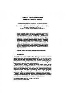
Making an accurate classifier ensemble by VCI Figure 1

5

Framework of VCI predictors (see online version for colours)

Note: Given an initial dataset (missing k% of the values), randomly generate n incomplete datasets by removing m% of the observed values n times; impute the missing values to generate n (slightly different) training sets, and then learn a classifier on each imputed dataset. To subsequently classify a new instance, have each classifier produce its classification, then return the most frequent classification.

2.3 Machine learning algorithms used In general, a learning algorithm takes as input a set of labelled instances and returns a classifier; that classifier in turn takes as input an unlabelled instance and returns a single label. Here, we consider the following ten algorithms L from WEKA (Witten and Frank, 2005). While each algorithm will see only complete (imputed) training instances within VCI(L, I(.)), the VCI(L, default) system will run L on incomplete data, using L’s default approach to dealing with incomplete data. We therefore summarise the base machine learning algorithms and how each of them handles incomplete data, below.

2.3.1 Decision table Decision table (dTable) is a set of schema/body pairs, where each schema is a set of attributes, and a body consists of labelled instances from the space defined by the features in the schema (Kohavi, 1995). Given an unlabelled instance, the dTable classifier searches for exact matches in the decision table only using the features in the schema. If it finds no such matching instances, it then returns the majority class; otherwise, it returns the majority class of all matching instances. DTable ignores missing values during the learning and classification processes.

2.3.2 Decision tree Decision tree (C4.5) grows decision trees from the root downward, greedily selecting the next attribute for each new decision branch added to the tree. Its various decisions, such

6


as which attribute to select and whether to stop, are based on information gain. Here, the C4.5 algorithm just ignores missing values. It classifies an instance by following the tree from the root to a leaf. If an instance reaches a node labelled with a feature that is missing, the decision will descend down all branches, but with a probability based on the percentage of training instances that went down that branch (Quinlan, 1993). The final classification will be the most likely outcome, based on the summed likelihood.

2.3.3 Decision list PART is a decision list classifier based on partial decision trees (does not do optimisation as decision tree does), which combines C4.5 and the RIPPER rule classifier (Cohen, 1995) for rule generation by creating rules from decision trees and the separate-and-conquer rule learning technique. PART deals with missing values using the same strategy as C4.5 (Frank and Witten, 1998).

2.3.4 Naïve Bayes NB is a simple Bayesian network that assumes attribute values are conditionally independent given the class. It typically assumes that numeric attributes obey a Gaussian distribution (John and Langley, 1995). NB learns by estimating the prior probability of each class and the conditional distributions of each attribute given the class. It simply ignores attribute values that are missing during both learning and classifying.

2.3.5 Logistic regression LR uses a multinomial LR model with a ridge estimator, and uses a ReplaceMissingValuesFilter to replace the missing values with the mean (for numeric attributes) or the most frequent value (for nominal attributes) (Le Cessie and van Houwelingen, 1992) during the training stage.

2.3.6 Random forest RF grows many classification trees and uses a voting scheme to determine the final classifications. To classify a new instance, it first asks each tree in the forest for its classification, and then takes the classification having the most votes. The RF learner replaces the missing values with the median value for numeric attributes or the most frequent value for nominal attributes. RF fills in the missing data in test set using filled-in values from the training set (Breiman, 2001).

2.3.7 One rule OneR is a rule-based classifier that infers one rule that predicts the class based on the most informative attribute. Each attribute is assumed to be discrete, otherwise it must be discretised. Missing values are treated as a new value, ‘missing’ (Holte, 1993).

2.3.8 Support vector machine A kernel-based SVM produces non-linear boundaries by constructing a linear boundary in a large, transformed (kernelised) version of the feature space. The SVM


7

implementation in WEKA uses the sequential minimal optimisation (SMO) algorithm (Platt, 1998) for training a support vector classifier using polynomial (which we used) or RBF kernels. This implementation globally replaces all missing values by a default value, for example ‘unknown’.

2.3.9 K nearest neighbour A kNN classifier finds the k labelled instances in the training data (‘neighbours’) that are nearest to the given unlabelled instance, and returns the average value of the real-valued labels of the neighbours, and the most frequent label for nominal ones. The distance of the neighbours is defined in terms of Euclidean distance for continuous attributes and Hamming distance for discrete ones. KNN handles missing values by means of a minor change in the distance measure: when the two instances each miss the values of the same attribute, the distance on that attribute is zero, but when only one has a missing value, a maximal distance is assigned (Witten and Frank, 2005).

2.3.10 Neural network A NN is composed of interconnected input/output units, where each connection has an associated weight, typically learned by the backpropagation algorithm. Many NN models have been modified to handle missing data. Following (Ishibuchi et al., 1993), we replace each missing value by an interval that includes all of the possible values on that attribute (e.g. a unit interval [0, 1]), and also replace each observed value by a degenerate interval (e.g. 0.7 transformed to [0.7, 0.7]), before applying the backpropagation algorithm. Learning and making classification from incomplete data are therefore turned to classification of the (complete) interval vectors.

2.4 Imputation methods used After removing a small percentage of attribute values, VCI uses some imputation techniques to fill in the missing information. This subsection summarises five such imputers.

2.4.1 Mean imputation MEI fills in each missing value with the mean of the values observed values for the corresponding attribute,

θ MEI =

1 | U (i ) |

∑

Y u∈U (i ) u , i

(1)

where each instance u ∈ U(i) has an observed values of attribute i. Many machine learning algorithms use MEI as it is an extremely simple imputation technique. Unfortunately, it is problematic as it can distort the shape of distributions by creating a spiked distribution at the mean in frequency distributions, which attenuates the correlation of the associated item with others; and it also reduces (underestimates) the variance of the predictions which generally leads to incorrect inferences.

8


2.4.2 Bayesian multiple imputation Standard single imputation produces a single imputed dataset where each missing value is replaced with a single value. While this approach can be applied to virtually any dataset, single imputation does not account for the uncertainty about the predictions of the imputed values; this can lead to statistically invalid inferences (Rubin, 1987). By contrast, multiple imputation (MI) produces many different imputed datasets. For example, consider imputing a value in the (2, 1) position in the left 5 x 3 table in Figure 2 (here the entry (i, j) is the value of the jth feature of the ith instance Ri). Here, we could produce m = 4 different completed datasets, shown as the middle column of four tables in that figure; note the proposed values for this (2, 1) entry are {1, 1, 3, 3}. BMI uses the average of these four values (here, 2) as the final prediction – see the right 5 x 3 table in the figure. In many situations, MI approaches have proven to be highly effective even for small values of m – say 3–15 (Rubin, 1987). BMI follows a Bayesian framework: it specifies a parametric model for the complete data, with a given a priori distribution over the unknown model parameters θ, then simulates m independent draws from the conditional distribution of the missing data given the observed data. While BMI assumes a multivariate normal distribution when generating the imputations for missing values, it is robust to non-normally distributed data (Schafer, 1997). In non-trivial applications, special computational processes, like Markov chain Monte Carlo (MCMC), must be applied to perform BMI (Rubin, 1987). BMI imputes data as follows (Rubin, 1987): Let P(Ycom|θ) model the complete data based on the parameter θ (which here is the mean and covariance matrix that parameterises a normal distribution). If Y = (Yobs, Ymiss) follows a parametric model P(Y|θ) where θ has the prior distribution P(θ), then the posterior predictive distribution for Ymiss is

∫

P (Ymiss | Yobs ) = P (Ymiss | Yobs ,θ ) P (θ | Yobs ) dθ Figure 2

An example of BMI with m = 4

Note: Each value in the shaded cells is an imputed value. BMI produces different imputed datasets (the middle tables) and takes the average of the m predictions as the final imputed dataset (the right table).

(2)


9

Equation (2) suggests that BMI can be drawn by iterating the following process for j = 1, …, n: 1

generate missing values Ymiss(j+1) from P(Ymiss|Yobs, θ (j))

2

draw parameters fromθ (j+1) from P(θ|Yobs, Ymiss(j+1)).

Repeat these two steps to generate the Markov chain {Ymiss(1), θ (1), Ymiss(2), θ (2), …, Ymiss(j), θ (j), …}; note that Ymiss(j+1) depends on θ (j) and θ (j) depends on Ymiss(j). This entire process is repeated until the distribution P(Ymiss, θ |Yobs) is stabilised (Schafer, 1997). After producing m sets of filled-in values, BMI takes the average as the final imputed values,

θ=

1 m

m ∧

∑θ

(3)

i

i =1

where θî is the imputation in the ith set of imputed values. We round the BMI imputed values to the nearest integers for integer attributes. We also find the observed value range [min, max] for each attribute, and replace imputed values < min with min, and those > max with max for missing values. We also apply this post-processing procedure to the other imputers described below.

2.4.3 Linear regression imputation LinR imputation predicts the missing value of one attribute based on the observed values of other attributes. In general, given a one-dimensional vector of inputs X = (X1, X2, …, Xp), LinR estimates the dependent value Y based on the LinR model p

Y = β0 +

∑X β j

j

+ε

(4)

j =1

where the residual ε is a random variable with mean zero, and the coefficients β0 and

β = (β1, β2, …, βp)T are trained on the existing values to minimise the L2 norm (square root of the sum of the squares of the residuals) (Spaeth, 1991). Here, Y is the missing feature value to be imputed and each Xj is the value of an observed feature of the same instance. To illustrate, consider again the simplified example in the upper left table of Figure 2, which corresponds to five instances, each involving three features. To estimate r(2, 1), notice the instance R2 has observed values for attributes A2 and A3. The LinR imputer would first find all other instances that have observed values for these attributes, and also A1 (the attribute we want to predict a value for); this identifies instances R(A1, A2, A3) = {R1, R4, R5}. LinR then seeks coefficients β0, β2 and β3 such that r(Ri, A1) = β0 + β2r(Ri, A2)+β3r(Ri, A3). Using this data subset {r(Uj, Ik)|j ∈ {1, 4, 5}, k ∈ {1, 2, 3}}, the best-fit line has β0 = −1, β2 = 0 and β3 = 1. LinR now computes its prediction for r(R2, A1) = β0 + β2r2, 2 + β3r2, 3 = 2. Here, there were three equations (for R1, R4, R5) and three unknowns {β0, β2, β3} which produces this unique solution. In other situations, there might be more equations than unknowns; here, we use standard linear least square estimate (Spaeth, 1992).

10


2.4.4 Expectation maximisation imputation EM seeks maximum likelihood estimates of parameters in probabilistic models in the presence of latent variables (Dempster et al., 1977). EM imputation requires specifying a joint probability distribution for the feature value to be imputed and other feature values. EM iterates between performing an expectation E-step, which calculates an expected value of the complete data likelihood, given the observed data and the current parameters; and a maximisation M-step, which computes values of the parameters that maximise the expected likelihood over the data including those estimated in the E-step. The parameters found on the M-step are then used to begin another E-step, and the process is repeated until it converges to a stationary point. Our implementation of the EM algorithm, like BMI, assumes the data follows a multivariate Gaussian distribution (parameterised by the mean and the covariance matrix), and uses a ridge regression (Schneider, 2001). It first produces an initial guess of these parameters. In each subsequent iteration, EM updates its estimates of the mean and the covariance matrix in the following two steps (Schneider, 2001): 1

E-step: replace the missing values in an instance with their conditional expectation values given the observed values using the estimated mean and covariance matrix.

2

M-step: re-estimate the mean and the covariance, using the instance mean of the completed dataset and the covariance matrix as the sum of the instance covariance matrix of the completed dataset and the contributions from the conditional covariance matrix of the imputation errors.

EM iterates these steps until the imputed values and the estimates of the mean and covariance stop changing (Little and Rubin, 1987).

2.4.5 Predictive mean matching imputation PMM (Landerman et al., 1997) imputes the missing values Ymiss, i of an incomplete instance (recipient) Yi, based on the observed part of that instance Yobs, i using a distance function (Equation (6)) that is computed as the expected values of the missing variables conditioned on the observed covariates, instead of directly on the values of the covariates. Our version of PMM works as follows: 1

Use the EM algorithm (Dempster et al., 1977) to estimate the parameters θ of a multivariate Gaussian distribution over the attribute values using all the available data.

2

Based on these estimates, compute the conditional expected value for the missing part Ymiss, i of instance Yi conditioned on the observed part Yobs, i based on the estimated parameters θ ∧

μ i = E (Ymiss, i | Yobs, i ,θ ) . 3

(5)

Each recipient Yi is matched to the instance (possible donor) Yj = argminj d(i, j) that has the nearest predictive mean with respect to the Mahalanobis distance, d (i, j ) =

( μî − μˆ j ) S Y T

−1 miss, i |Yobs, i

( μî − μˆ j )

(6)

Au: Please check this sentence ‘EM imputation requires …’ under Section 2.4.4 as it appears it may be incomplete.

Making an accurate classifier ensemble by VCI where

S

−1 Ymiss, i |Yobs, i

11

is the residual covariance matrix from the regression of the missing

items on the observed ones (Landerman et al., 1997). 4

Impute missing values in each recipient using the corresponding values from its closest donor.

In the example in the upper left table of Figure 2, PMM first uses EM to estimate the values of each missing instance – for example, for the incomplete instance (recipient) Y2, PMM computes the predictions of the missing feature values, Ymiss, 2 = {r(2, 1)}, conditioned on the observed feature values Yobs, 2 = {r(2, 2), r(2, 3)} = {4, 3}, of the entire row associated with the instance Y2. The same predictive means are computed for all the possible donors Yj, that is, Yj = {r(j, 1), r(j, 2), r(j, 3)} where this j varies over all instances except the recipient Y2. The recipient Y2 is then matched to the donor that has the closest predictive mean in terms of the Mahalanobis distance, which here is Y1 = {r(1, 1), r(1, 2), r(1, 3)}; hence the missing value r(2, 1) is imputed by taking the corresponding value r(1, 1) = 2 from Y1.

3

Experimental design and results

3.1 Preliminary experiments on imputation techniques Before applying the imputation techniques into VCI predictors, we first investigated the effectiveness of the imputers, including MEI, BMI, LinR, PMM and EM. We work on the UCI machine learning repository dataset ‘letter’, which has 20,000 samples and 16 attributes, each of which ranges over the values {0, 1, 2, …, 15}. We randomly remove values from the dataset to generate eight datasets, with missing ratios of 10%, 20%, …, 80%. By applying the imputation techniques, we compare the imputed values with the ground truth, and calculate the respective root mean square error (RMSE) of these imputed values on this specific dataset. RMSE =

1 n

∑ (p {u , i}

u,i

− ru , i

)

2

(7)

where n is the total number of estimated values by an imputer, pu, i is the imputed value for instance u on attribute i and ru,i is the ground truth value. Table 1 and Figure 3 show that EM and BMI perform the best on this dataset. MEI has almost stable accuracy on datasets with different missing ratios (it is therefore relatively worse for dense datasets and relatively better for sparse ones), and the other two imputation techniques, PMM and LinR, fall far behind. Although second to the EM imputer, the BMI imputer is robust to datasets with missing ratio higher than 50%, for which EM often fails to produce imputations due to an eigenvalue calculation exception (this is why Figure 3 includes only the EM results for datasets with missing ratios at most 50%).

12 Table 1 Ratio%

X. Su, T.M. Khoshgoftaar and R. Greiner The RMSE performance of the imputation techniques on the dataset ‘letter’ with different missing ratios BMI

EM

PMM

LinR

MEI

10

1.7017

1.5089

2.2699

2.2653

2.3249

20

1.7516

1.6557

2.3627

2.3580

2.3346

30

1.8066

1.7090

2.4194

2.4115

2.3297

40

1.8637

1.7677

2.5147

2.5057

2.3264

50

1.9325

1.8203

2.5992

2.5916

2.3339

60

2.0042

NA

2.7114

2.7127

2.3292

70

2.1008

NA

2.8481

2.8451

2.3293

80

2.2424

NA

2.9941

2.9905

2.3301

Figure 3

The RMSE performance of the imputation techniques on the dataset ‘letter’ with different missing ratios (see online version for colours)

BMI is also very efficient, requiring only about 5 min to impute the dataset ‘letter’ (on our computer with a 3.2 GHz Intel CPU and 4 GB RAM) at the missing ratio of 50%. However, PMM and EM require more than 20 min each using the same machine. Based on the above preliminary experiments, we dropped the imputation techniques PMM and LinR from further experiments.

3.2 Experimental design We apply our proposed VCI(L, I(.)) system using the I(.) ∈ {MEI, BMI, EM} imputation techniques. We investigated VCI predictors on both complete datasets and incomplete datasets. We worked on ten datasets with numeric or ordinal attributes from the UCI machine learning repository (Blake and Merz, 2000; see Table 2) (We focus on this class of data as each of these imputers only deals with numeric and ordinal data, but not categorical data). We applied each of the ten base learners L introduced in Section 2.3, in general, using the default parameters given by WEKA. We used 50 trees for the RF classifier and


13

used k =5 as the number of neighbours for the kNN classifier, which produced optimal performance in our preliminary experiments. When implementing our proposed imputers, BMI and EM iterate until they converge. For example, on the dataset ‘letter’ with 30% missing ratio, BMI needs nine iterations to converge while EM needs six. When preprocessing the incomplete data with an imputer, we impute the training and test sets together. Notice, none of the imputers use the class labels of the test sets. (Our empirical results show that classifying on the imputed test data (excluding class labels) slightly but insignificantly outperforms classifying on the original incomplete test data.) We used the standard training and test splits for each of these UCI datasets: 2/3 of the instances for training and 1/3 for testing, except the dataset ‘letter’, where we used a 3/4 to 1/4 split, and the dataset ‘waveform’, where we trained on 300 instances and tested on 4,700. How many learning sets should VCI produce for each dataset? We know that small numbers may incur high biases and large numbers will increase computational expense. We want an odd number in order to break ties in voting, especially for binary class datasets. Therefore, we focussed on 7 ~ 11 and decided to use n = 9. To compare, we also use n = 9 bootstrap learning sets for the bagging predictors, which performs similarly to the WEKA default setting of n = 10. We formed each such learning dataset by randomly removing 3% of the attribute values (see the discussion in Section 3.4). Table 2 Datasets Australian

Description of the datasets used in our experiments #Train 460

#Test

#Attribute

#Class

230

14

2

Breast-wisc

466

233

10

2

Diabetes

512

256

8

2

Heart

180

90

13

2

Letter

15,000

5,000

16

26

Pima

512

256

8

2

Satimage

4,290

2,145

36

6

Segment

1,540

770

19

7

Vehicle

564

282

18

4

Waveform

300

4,700

21

3

3.3 VCI predictors on complete datasets We first investigate VCI predictors on complete data (i.e. the special case of ‘incomplete data’ with missing ratio of 0%) on the ten datasets described in Table 2. Table 3 and Figure 4 show the classification accuracy of VCI(L, …) predictors as well as the original classifier L and bagging, over all ten complete datasets. We see that VCI improves average classification accuracy over the base classifiers L except NB, RF and LR. Over all base learners L, VCI(L, EM) and VCI(L, BMI) perform significantly better than the original learners L with one-sided t-test p < 0.01 and p < 0.008, respectively. VCI(L, EM) insignificantly outperforms bagging predictors with p < 0.1. Other VCI predictors also outperform the original classifiers, and perform slightly better than or equivalent to bagging predictors.

14 Table 3

X. Su, T.M. Khoshgoftaar and R. Greiner Average classification accuracy of VCI predictors over ten UCI complete datasets

Base learners

Original classifiers

Bagging

VCI default

VCI MEI

VCI EM

VCI BMI

OneR

67.10

68.10

68.50

68.39

68.56

68.50

NB

76.97

76.79

76.31

75.99

76.10

76.03

DTable

81.14

82.84

82.01

82.63

82.91

82.27

C4.5

85.19

86.83

87.10

86.90

86.76

86.89

KNN

85.76

84.64

85.93

86.35

86.76

86.58

PART

84.98

86.45

87.76

86.98

87.43

86.98

SVM

84.41

85.59

84.54

84.69

84.94

85.31

LR

85.70

85.73

85.70

85.67

85.63

85.99

NN

85.35

86.92

86.29

87.13

87.32

86.50

RF

88.11

87.12

87.56

87.51

87.90

87.93

Average

82.47

83.10

83.17

83.22

83.43

83.30

Figure 4

Average classification accuracy of VCI predictors over ten UCI complete datasets (see online version for colours)

Note that VCI(L, default), which uses each L’s default method to deal with missing values (described in Section 2.2), significantly outperforms original classifiers L with p < 0.037.


15

3.4 VCI predictors on incomplete datasets We have shown that VCI works on complete data; now, we experiment to see if it also works on incomplete data. We first present our results on incomplete datasets generated from the complete datasets (see Table 2) by randomly deleting 30% of the observed values. We then report results on the dataset ‘waveform’, with missing ratios of 10%, 20%, …, 50% to investigate performance of VCI predictors on incomplete data with different missing ratios. We finally explore the effects of the injected missing ratio m% on the predictive accuracy of VCI predictors. From Table 4 and Figure 5 (see Appendix for more detailed results of VCI predictors with each base learner L on every dataset), we found VCI(L, BMI) and VCI(L, EM) significantly outperform original learners L by 10.2% and 9.7% higher average classification accuracy (with p < 0.0032 and p < 0.0042, respectively); VCI(L, BMI) and VCI(L, EM) perform significantly better than bagging predictors with 9.4% and 9.0% higher average classification accuracy (with p < 0.026 and p < 0.032, respectively). To compare, we also implemented imputation-helped learners (machine learners that learn classifiers on imputed training data instead of originally incomplete data) (Su et al., 2008), and found VCI(L, BMI) outperforms BMI-imputed machine learners (imputationhelped learners using BMI as the preprocessor for incomplete data) with 3.0% higher average classification accuracy (p < 0.00065); VCI(L, EM) has 1.7% higher average accuracy than EM-imputed machine learners (p < 0.015). VCI(L, MEI) outperforms MEI-imputed machine learners with 7.2% better accuracy (p < 0.018), and it outperforms the original classifiers and bagging predictors with 4.5% and 3.8% better average classification accuracy, respectively (with p < 0.049 and p < 0.17, respectively). VCI(L, I(.)) predictors greatly improve classification accuracy on incomplete data for almost all of the respective machine learned classifiers L, we investigated in this work, including the stable learners kNN and RF, which regular ensemble classifiers such as bagging fail to improve. VCI using BMI and EM on kNN (VCI(kNN, BMI) and VCI(kNN, EM)) have 39.5% and 39.3% accuracy improvements, respectively, over the original kNN classifier. We believe this is due to the crude way that kNN handles missing data (see Section 2.3), and the observation that imputed values can be better used for distance calculation than the missing values. Moreover, voting on the classifications from the diverse imputed learning sets further improves the performance. On another stable learner, NB, however, VCI(NB, I(.)) predictors perform slightly worse. This is because NB classifies an instance by computing the class with maximum probability given the observed values, while imputing diverse learning sets and voting based on their classifications often do not provide better inference for NB. We investigated the performance in terms of accuracy of VCI predictors on the dataset ‘waveform’ with missing ratios 10–50%. Table 5 and Figure 6 show that VCI(L, BMI) and VCI(L, EM) dominate over their rivals, and enlarge their advantage on datasets with higher missing ratios. VCI(L, default) predictors (that use the default simple ways to handle incomplete data) and MEI-imputed machine learners perform equivalently with bagging predictors; and VCI(L, MEI) predictors perform better than bagging predictors. BMI-imputed and EM-imputed machine learners perform better than the original classifiers, bagging predictors and VCI(L, MEI), but inferior to VCI(L, BMI) and VCI (L, EM).

16


Table 4

Average classification accuracy of VCI predictors over ten UCI incomplete datasets with 30% missing ratios

Base learners

Original classifier

Bagging

OneR

56.33

59.09

56.41

63.26

NB

73.35

73.58

71.59

DTable

66.35

65.36

71.96

LR

75.03

74.36

SVM

74.68

74.82

NN

70.72

C4.5

73.93

kNN PART

VCI-EM

VCI-BMI

63.75

63.95

64.44

72.18

72.66

72.54

72.55

72.99

74.20

75.72

76.11

74.49

76.94

78.00

78.21

78.57

75.17

78.04

78.60

78.69

79.52

74.77

76.58

78.14

77.81

79.61

79.86

77.63

76.64

75.54

76.52

80.74

80.38

57.61

48.38

74.41

78.56

79.50

80.25

80.39

75.12

79.88

77.75

76.49

76.87

80.71

81.3

RF

80.18

80.45

80.03

80.51

81.03

81.33

81.76

Ave

70.33

70.83

73.50

75.26

75.89

77.17

77.49

Figure 5

VCI-MEI BMI-impute EM-impute

Average classification accuracy of VCI predictors over ten UCI incomplete datasets with 30% missing ratios (see online version for colours)

Making an accurate classifier ensemble by VCI Table 5

17

Average classification accuracy of VCI predictors over ten classifiers on the dataset ‘waveform’ with missing ratios 10–50%

Predictors

10%

20%

30%

40%

50%

Original classifiers

72.86

71.21

68.3

66.67

63.91

Bagging predictors

74.98

73.44

69.67

68.47

64.63

BMI-imputed

75.37

75.22

74.88

73.51

72.03

EM-imputed

75.56

75.51

75.81

73.31

73.69

MEI-imputed

73.43

72.5

69.97

67.73

66.19

VCI-BMI

77.76

77.75

77.28

76.51

74.21

VCI-EM

77.52

77.42

77.19

75.79

74.49

VCI-default

74.83

73.1

69.53

68.13

65.5

VCI-MEI

75.95

75.03

71.57

70.05

68.14

Figure 6

Average classification accuracy of VCI predictors over ten classifiers on the dataset ‘waveform’ with missing ratios 10–50% (see online version for colours)

To investigate the impact of injected missing ratios on VCI predictors, we applied VCI(L, EM) to the ‘waveform’ dataset that has a 30% original missing ratio, and additionally removed observed values with injected missing ratio m% = 1–9%. The results (see Figure 7) show that, for most learners L, VCI(L, EM) with injected missing ratios ≥ 3% perform similarly to each other (with different m%). VCI(C4.5, EM) and VCI(dTable, EM) have better classification accuracy with higher injected missing ratios over the above injected missing ratio span. As the classification accuracy of VCI predictors and other classifiers generally decrease with higher missing ratios, we did not consider an injected missing ratio ≥ 8%. We therefore recommend an injected missing ratio between 3% and 8%; here, we used 3%.

18


Figure 7

Impact of injected missing ratios on VCI predictors: VCI-EM on the ‘waveform’ dataset with 30% missing ratio and different injected missing ratios (see online version for colours)

The computational expense for VCI predictors is imputation_time + training_time for preprocessing and training time, and classifying_time × number_of_learning_sets + voting_time for performance time. The ‘number of learning sets’ factor is standard for ensemble classifiers (such as bagging, boosting). Here, the extra expense is the imputation time. As we mentioned in Section 3.1, the imputation for the biggest dataset in our experiments, ‘letter’ (with 30% missing data), using BMI takes only a few minutes. For most mid-sized or small-sized datasets, the imputation time is ignorable. As missing data that are not missing at random (NMAR) are usually problem specific, we did not experiment on datasets with this missing mechanism. We plan to investigate the impact of using these imputation techniques for incomplete data that are missing at random (MAR, whose missingness depends on observed values but not on unobserved ones) in our future work. We also plan to investigate VCI predictors on categorical data in our future work.

4

Conclusions

We propose a novel ensemble approach, VCI, that produces many diverse learning sets by first removing observed attribute values multiple times and then imputing the resulting incomplete learning sets using state-of-the-art imputation techniques, such as BMI and EM. It then uses a base learner to learn a classifier for each imputed learning set. Our empirical studies show that VCI predictors (whose classification is the plurality over the individual classifiers) can significantly improve the classification accuracy over conventional classifiers, especially for incomplete datasets with high missing ratios.


19

VCI(L, BMI) (VCI using BMI as the imputer, and a base learner L) and VCI(L, EM) significantly outperform most of the respective machine learned classifiers L we investigated, including kNN, NN, OneR, decision table, SVM, LR, decision tree (C4.5), RF and decision list (PART). VCI predictors also have significantly better performance than the well-known bagging predictors and imputation-helped machine learners, and perform especially well for the stable process kNN where bagging fails to improve accuracy.

References Blake, C. and Merz, C. (2000) UCI Repository of Machine Learning Databases. Available at: http://www.ics.uci.edu/~mlearn/MLRepository.html. Breiman, L. (1996) ‘Bagging predictors’, Machine Learning, Vol. 24, p.2. Breiman, L. (2001) ‘Random forests’, Machine Learning, Vol. 45, No. 1, pp.5–32. Cohen, W. (1995) ‘Fast effective rule induction’, Proceedings of the 12th International Conference on Machine Learning (ICML), pp.115–123. Dempster, A.P., Laird, N.M. and Rubin, D.B. (1977) ‘Maximum likelihood from incomplete data via the EM algorithm’, Journal of the Royal Statistical Society, Vol. B39, pp.1–38. Frank, E. and Witten, I.H. (1998) ‘Generating accurate rule sets without global optimization’, Proceedings of the 15th International Conference on Machine Learning (ICML), pp.144–151. Freund, Y. and Schapire, R.E. (1997) ‘A decision-theoretic generalization of on-line learning and an application to boosting’, Journal of Computer and System Sciences, Vol. 55, No. 1, pp.119–139. Holte, R.C. (1993) ‘Very simple classification rules perform well on most commonly used datasets’, Machine Learning, Vol. 11, pp.63–91. Ishibuchi, H., Miyazaki, A., Kwon, K. and Tanaka, H. (1993) ‘Learning from incomplete training data with missing values and medical application’, Proceedings of 1993 International Joint Conference on Neural Networks (IJCNN), pp.1871–1874. John, G.H. and Langley, P. (1995) ‘Estimating continuous distributions in Bayesian classifiers’, Proceedings of the 11th Conference on Uncertainty in Artificial Intelligence (UAI), pp.338–345. Kohavi, R. (1995) ‘The power of decision tables’, Proceedings of the 8th European Conference on Machine Learning (ECML), pp.174–189. Kuncheva, L. and Whitaker, C. (2003) ‘Measures of diversity in classifier ensembles and their relationship with the ensemble accuracy’, Machine Learning, Vol. 51, p.2. Landerman, L.R., Land, K.C. and Pieper, C.F. (1997) ‘An empirical evaluation of the predictive mean matching method for imputing missing values’, Sociological Methods and Research, Vol. 26, pp.3–33. Le Cessie, S. and van Houwelingen, J.C. (1992) ‘Ridge estimators in logistic regression’, Applied Statistics, Vol. 41, No. 1, pp.191–201. Little, R.J.A. and Rubin, D.B. (1987) ‘Statistical analysis with missing data’, Series in Probability and Mathematical Statistics, Wiley, p.278. Melville, P. and Mooney, R.J. (2004) ‘Creating diversity in ensembles using artificial data’, Journal of Information Fusion, Vol. 6, No. 1, pp.99–111. Platt, J. (1998) ‘Fast training of support vector machines using sequential minimal optimization’, Advances in Kernel Methods Support Vector Learning, pp.185–208. Quinlan, J.R. (1993) C4.5: Programs for Machine Learning. Los Altos: Morgan Kaufmann. Rubin, D.B. (1987) Multiple Imputation for Non response in Surveys. New York, NY: J. Wiley & Sons.

20


Schafer, J.L. (1997) Analysis of Incomplete Multivariate Data. New York, NY: Chapman and Hall. Schneider, T. (2001) ‘Analysis of incomplete climate data: estimation of mean values and covariance matrices and imputation of missing values’, Journal of Climate, Vol. 14, pp.853–871. Späth, H. (1992) Mathematical Algorithms for Linear Regression. Boston, MA: Academic Press. Su, X., Khoshgoftaar, T.M. and Greiner, R. (2008) ‘Using imputation techniques to help learn accurate classifiers’, The 20th IEEE International Conference on Tools with Artificial Intelligence (ICTAI), Dayton, Ohio, USA, November. Su, X., Khoshgoftaar, T.M. and Zhu, X. (2008) ‘VCI predictors: voting on classifications from imputed learning sets’, The IEEE International Conference on Information Reuse and Integration (IRI), pp.296–301. Witten, I.H. and Frank, E. (2005) Data Mining: Practical Machine Learning Tools and Techniques (2nd ed.), San Francisco, CA: Morgan Kaufmann. Zhang, Y., Zhu, X. and Wu, X. (2006) ‘Corrective classification: classifier ensembling with corrective and diverse base learners’, Proceedings of the 6th IEEE International Conference on Data Mining (ICDM), pp.1199–1204. Zhang, Y., Zhu, X., Wu, X. and Bond, J.P. (2005) ‘ACE: an aggressive classifier ensemble with error detection, correction and cleansing’, Proceedings of the 17th IEEE International Conference on Tools with Artificial Intelligence (ICTAI), pp.310–317.


21

Appendix Complete results of VCI predictors with each classifier on each incomplete dataset with 30% missing ratios Table A1

Classification accuracies of the original classifiers

Classifiers DTable

NB

OneR

C4.5

kNN

PART SVM

LR

NN

RF

Ave

Australian

76.96 76.09

74.35 77.39 79.13 83.48 75.22 78.26 75.22 82.61 77.87

Breast

91.85 95.71

86.70 91.42 89.70 93.56 94.85 94.42 90.56 96.57 92.53

Diabetes

68.36 68.36

68.36 67.97 58.20 65.63 69.53 69.53 65.63 67.97 66.95

Heart

68.89 88.89

66.67 81.11 73.33 81.11 87.78 87.78 81.11 82.22 79.89

Letter

34.50 54.28

12.76 55.14 7.140 57.62 51.68 49.66 45.66 73.10 44.15

Pima

69.14 75.00

72.66 71.09 58.20 68.36 76.17 77.73 67.19 75.39 71.09

Satimage

68.72 78.23

45.92 80.19 51.52 82.89 81.49 80.84 83.08 84.80 73.77

Segment

74.94 79.22

47.79 85.58 81.82 87.14 77.79 78.70 74.81 92.08 77.99

Vehicle

52.84 39.36

41.84 60.28 24.11 60.64 53.19 56.03 48.58 70.57 50.74

Waveform

57.28 78.32

46.23 69.17 52.91 70.77 79.13 77.38 75.32 76.45 68.30

Average

66.35 73.35

56.33 73.93 57.61 75.12 74.68 75.03 70.72 80.18 70.33

Table A2

Classification accuracies of the bagging predictors

Bagging

DTable

Australian

80.00

NB

OneR

C4.5

kNN

PART SVM

LR

NN

RF

Ave

75.22 74.35 84.35 76.09 85.22 75.65 78.26 77.83 82.61 78.96

Breast

92.70

95.71 87.12 95.28 87.12 97.00 95.28 94.42 93.99 96.14 93.48

Diabetes

65.63

67.97 67.58 66.41 57.03 67.97 69.14 69.14 67.58 68.36 66.68

Heart

71.11

88.89 72.22 82.22 70.00 85.56 86.67 85.56 82.22 84.44 80.89

Letter

28.42

54.86 15.48 66.40 8.700 69.10 53.60 50.12 58.38 72.32 47.74

Pima

65.63

75.78 73.83 71.09 55.86 75.39 76.17 77.73 73.83 76.17 72.15

Satimage

71.19

78.09 46.20 81.96 23.36 84.99 81.72 81.07 84.20 84.85 71.76

Segment

84.29

79.61 59.22 88.44 36.10 90.26 78.57

Vehicle

33.69

41.13 43.26 65.25 25.89 67.02 52.13 55.67 53.90 69.50 50.74

NA

78.57 92.99 76.45

Waveform

60.91

78.53 51.64 74.85 43.64 76.32 79.23 77.23 77.23 77.09 69.67

Average

65.36

73.58 59.09 77.63 48.38 79.88 74.82 74.36 74.77 80.45 70.83

22


Table A3

Classification accuracies of the VCI predictors using BMI

VCI-BMI

dTable

Australian

79.57 78.26 79.57 81.30 81.74 81.74 79.13 81.74 81.30 82.61 80.70

NB

OneR

C4.5

kNN

PART

SVM

LR

NN

RF

Ave

Breast

95.28 93.99 92.27 95.71 95.28 96.57 95.71 95.28 95.71 96.14 95.19

Diabetes

71.88 68.75 72.66 73.83 66.80 71.88 69.14 68.36 67.97 71.88 70.32

Heart

85.56 88.89 77.78 83.33 87.78 85.56 86.67 86.67 82.22 86.67 85.11

Letter

45.88 48.72 15.88 67.84 72.18 69.14 58.80 55.76 64.02 74.36 57.26

Pima

74.61 75.39 75.39 76.95 74.61 75.39 78.13 77.73 74.61 76.17 75.90

Satimage

84.06 78.41 56.60

88.3

89.79 89.23 84.57 88.18 88.81 90.12 83.81

Segment

84.55 75.58 64.68 88.83 88.96 90.39 95.58 86.33 88.18 90.26 85.33

Vehicle

62.77 38.65 51.77 69.50 67.38 73.40 65.60 66.31 75.89 68.44 63.97

Waveform

76.89 78.85 57.81 78.17 79.38 79.72 81.85 79.36 79.89 80.91 77.28

Average

76.11 72.55 64.44 80.38 80.39 81.3

Table A4

Classification accuracies of the VCI predictors using EM

VCI-EM

dTable

Australian

81.30

NB

OneR

C4.5

kNN

79.52 78.57 79.86 81.76 77.49

PART SVM

LR

NN

RF

Ave

76.96 80.43 81.74 81.74 82.61 80.43 80.87 82.17 80.87 80.91

Breast

94.42

94.85 93.99 96.14 95.28 95.28 95.71 95.71 95.28 96.14 95.28

Diabetes

70.70

69.92 74.22 70.70 68.36 73.44 69.14 68.75 66.80 71.09 70.27

Heart

85.56

88.89 78.89 85.56 86.67 83.33 85.56 85.56 82.22 85.56 84.78

Letter

46.62

48.66 14.36 64.36 71.10 68.44 59.12 55.14 63.36 72.28 56.34

Pima

73.83

75.00 73.83 72.66 75.00 76.56 78.91 77.34 75.78 76.56 75.55

Satimage

83.45

78.41 56.88 88.16 89.79 88.72 84.80 83.31 88.81 90.30 83.26

Segment

82.73

76.1

Vehicle

62.41

37.94 47.52 71.99 67.02 71.63 65.96 68.44 75.53 69.86 63.83

63.90 87.53 88.31 86.88 85.19 87.40 85.97 89.09 83.31

Waveform

76.17

78.64 55.49 78.53 79.26 80.21 82.04 79.62 80.13 81.55 77.16

Average

75.72

72.54 63.95 80.74 80.25 80.71 78.69 78.21 79.61 81.33 77.17