Transient Response Assessment of Vector PI Current

Transient Response Assessment of Vector PI Current Controllers in Renewable Energy Applications ´ Ana Vidal, Francisco D. Freijedo† , Alejandro G. Yepes, Jano Malvar, Oscar L´opez and Jes´us Doval-Gandoy Department of Electronics Technology, EII, Vigo, Spain (e-mail: anavidal, agyepes, janomalvar, olopez, [email protected]) † Gamesa Innovation and Technology, Madrid, Spain (e-mail: [email protected])

Abstract—Grid codes force generation units based on renewable sources to act similarly to conventional power plants: when a fault is detected, they must remain connected and support the grid. To fulfill these requirements, the transient response of the current controllers is critical. This paper applies a recently proposed methodology which assesses and optimizes the transient response of proportional-resonant controllers (PR) to a different type of linear regulators: the vector proportional-integral (VPI) controllers. This methodology is based on the study of the error signal roots: both reference tracking and disturbance rejection abilities should be considered for proper gain tuning. This work proves that VPI controllers lead to longer settling times and bigger overshoot than PR controllers for high sampling frequencies. However, as the sampling frecuency decreases, the transient response of both controllers presents more similarities. A three-phase voltage source converter prototype has been implemented. Experimental results provide a direct comparison between the transient behavior of VPI and PR controllers in different conditions: a +90 ◦ phase-angle jump in the current reference and a ‘type C’ voltage sag at the point of common coupling. Index Terms—Ac/dc power conversion, current control, dc/ac power conversion, distributed power generation.

I. I NTRODUCTION The increasing amount of renewable energy sources connected to the power system leads to problems to maintain voltage and frequency within the operating limits. In order to guarantee the stability and reliability of the utility network, the different countries have developped specific regulations called grid codes (GCs) [1]–[3]. Modern GCs force generation systems to remain connected to the network even when grid faults occur, which is known as low-voltage ride-through (LVRT) [4]. Moreover, during these events, the most demanding GCs also require generators to support the grid by supplying a certain amount of reactive power [1]–[3]. In renewable energy applications, the grid-side converter is usually based on dual-loop controllers [5], [6]. Inner loops with fast dynamics control the current according to the references given by the outer loops. These outer loops, which This work was supported by the Spanish Ministry of Science and Innovation and by the European Commission, European Regional Development Fund (ERDF) under Project DPI2009-07004.

978-1-4673-2420-5/12/$31.00 ©2012 IEEE

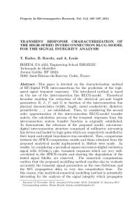
have slower dynamics, often regulate the reactive power and the dc-link voltage [5]. According to GCs, once a fault is detected, a certain amount of reactive current must be injected by the generation unit within a maximum delay [2], [3]. To fulfill this challenging requirement, two main tasks are critical: new reference generation and current control [6]. On the one hand, reference generation for the current control loop through outer power controllers with slower dynamics has to be disregarded [6]. On the other hand, the transient response of current controllers has to be optimized. Regarding this second task, a recent publication proposes a methodology to assess and optimize the transient response of proportional-resonant (PR) controllers [7]. It is based on the study of the error signal transfer function roots by means of pole-zero plots. Optimal gains are set to achieve fast and nonoscillating transient responses; i.e., to optimize the settling time. It is proved that optimal gain selection results from a tradeoff between transients caused by reference changes and transients caused by changes at the point of common coupling (PCC). The effect of different sampling frequencies fs is also discussed. According to this study, optimal tuning of PR controllers makes them suitable to fulfill the demanding GC requirements in terms of transient response. Vector proportional-integral (VPI) controllers are alternative resonant regulators to PR ones [8]–[10]. Some recent works show that VPI controllers could provide higher stability margins than PR ones, and hence, more damped responses [8]–[10]. Given these advantages of VPI controllers, and the lack of studies about their utilization in renewable energy applications, it seems appropriate to apply to them the methodology proposed in [7] and to compare the results to those obtained for the PR controller. Experimental results that allow the comparison between VPI and PR controllers transient behavior are included, regarding both reference and disturbance changes, as well as the effect of different fs . II. BACKGROUND A. Basic Concepts of Current Control Fig. 1 shows a block diagram of the current control loop [7], [11], where i and i∗ are the actual and the reference values of the current, respectively, e = i∗ − i denotes the error

5241

vPCC (t) i (k)

e (k)

*

+

‐

z -1

C (z)

PWM

+

‐

E∆v PCC (z) = F(s)

i (t)

i (k) DIGITAL CONTROLLER

Fig. 1.

F Tustin (z) ∆v PCC (z). 1 + C(z)z −1 F ZOH (z)

F Tustin (z) and F ZOH (z) are obtained by discretization of (1) with Tustin and ZOH methods, respectively. ∆i∗ (z) is discrete-time expression of a change (either in amplitude or in phase) in the current reference: ∆i∗ (z) =∆a

Block diagram of the current control closed-loop.

1 − z −1 cos(ωo0 Ts ) + 1 − 2z −1 cos(ωo0 Ts ) + z −2 | {z } cosine

signal and v PCC is the voltage at the PCC. C(z) represents a discrete-domain current controller. The block z −1 models the computational delay, while a zero-order hold (ZOH) is used for the pulse-width modulation (PWM). F (s) is the continuousdomain transfer function of the interface filter: 1 F (s) = (1) sLf + R with Lf being the filter inductance and with R being the equivalent resistance of the system. B. VPI Controllers VPI controllers are alternative resonant regulators to PR ones [8]–[10]. As resonant controllers, they have infinite gain at the resonant frequency, which assures steady-state perfect tracking and disturbance rejection for components pulsating at hωo , with ωo being the fundamental frequency and h being the harmonic order [8]–[10]. They can be expressed in the continuous-domain as follows: s2 Kph + sKih (2) C(s) = s2 + h2 ωo2 where Kph and Kih are the controller gains. VPI controllers provide very low gain for dc components [8]. Cancellation of the plant pole in (1) can be achieved by selecting the controller gains as Kph /Kih = Lf /R. Thus, (2) can be expressed as C(s) = Kh

s(sLf + R) s2 + h2 ωo2

(3)

where Kh = Kph /Lf . III. T RANSIENT A SSESSMENT BASED ON THE E RROR S IGNAL ROOTS This section summarizes the methodology proposed in [7]. It is based on the inspection of the pole-zero plots of the error signal caused by transients. The first step is the obtention of the discrete-time expression of the global error, which can be drawn from Fig. 1. As a linear system, the global error is the addition of the partial errors: E(z) = E∆i∗ (z) + E∆v PCC (z)

(4)

so that the error caused by reference changes E∆i∗ (z) and the error caused by disturbance changes E∆v PCC (z) can be analyzed separately. The discrete-domain transfer functions that represent the error in both situations are deduced: 1 ∆i∗ (z) (5) E∆i∗ (z) = −1 1 + C(z)z F ZOH (z)

(6)

z −1 sin(ωo0 Ts ) + ∆b 1 − 2z −1 cos(ωo0 Ts ) + z −2 | {z }

(7)

-sine

where ∆a and ∆b are the amplitude changes of the cosine and sine term, respectively. The same expression can be used for ∆v PCC (z), which models a voltage change at the PCC. In this work, C(z) is the discrete-domain expression of the VPI controller in (3), instead of a PR one (deeply analyzed in [7]). Discretization has been made decomposing (3) as the sum of two resonant terms and employing a different discretization method for each of them: Tustin with prewarping method for the sine term and impulse invariant method for the cosine term [9]. Once the error expressions are defined, one can graphically represent their roots and study their movement with gain variation, as well as the effects of their position in terms of transient response. The error transient response is, in this manner, optimized by making poles fast (large decay rates) and by placing them next to zeros that cancel their effect (small residues). IV. D ESIGN S TUDY The described methodology, applied to the VPI controller, is particularized for Lf = 4.51 mH and an equivalent series resistance Rf = 0.26 Ω. The same two transient tests as in [7] are analyzed: a phase change of +90 ◦ in the current reference (test I) and a typical sag in wind power intallations categorized as ‘type C’ with a characteristic voltage of the dip of 40% (test II). These two transients have been applied to a VPI controller tuned at the fundamental frequency with a fs = 10 kHz and a switching frequency fsw = 10 kHz in Section IV-A and with fs = fsw = 2.5 kHz in Section IV-B. It should be noticed that the VPI controller has only a gain to be tuned Kh [see (3)], unlike the PR one, which has two [7]. A. VPI Controller only at Fundamental Frequency Fig. 2 shows the variation in the pole placement with an increasing K1 in case of a reference change (test I) and a disturbance change (test II). With respect to the case described in [7], the study of the VPI controller implies to change only C(z), so just the roots that depend on this transfer function are different. Moreover, as the numerators and denominators of PR and VPI controllers are of the same order [9], the number of zeros and poles in (5) and (6) is the same for both controllers.

5242

1

1

0.5 /TS

0.1 0.2 0.3 0.4 0.5 0.6 0.7 0.8 = 0.9

0.8 0.6 0.4 0.2

z3

0

0.8

0.3 /TS

n

0.8 /TS

0.4

0.1 /TS

0.9 /TS

0.2

K1 p5-z4 p1

0.03 -0.4

z2 p3

0

-0.6

0.86 0.1

0.2

0.3

0.4

0.5

0.6

0.7

p3

0.8

0.9

-1

1

-1

-0.6

-0.8

(a) Test I. Roots of E∆i∗ (z).

-0.4

zoom

1.02

0.96

0.86

1

0.1 /TS

p6-z5

p2

-0.03

-0.8

0.96

p5-z4 z1

p7 -z2

0

0.2 /TS

p4

p1

0.03

-0.6

p6-z5

p2

z6

-0.2 -0.4

z1

-0.03

-0.8

zoom

0.3 /TS

K1

z3

/TS

0

p4

0

0.7 /TS

0.6

0.2 /TS

-0.2

-1

n 0.5 /TS 0.4 /TS 0.1 0.2 0.3 0.4 0.5 0.6 0.7 0.8 = 0.9

0.6 /TS

0.4 /TS

-0.2

0

0.2

0.4

0.6

0.8

1

(b) Test II. Roots of E∆v PCC (z).

Fig. 2. Pole-zero plot of the error signal during transients when using a single VPI controller at the fundamental frequency at fs = 10 kHz. Arrows indicate the variation of the pole placement when K1 increases from 50 to 1400. The poles and zeros that are cancelled with each other are shown in gray.

1

0.5 /TS

0.4

0

p4VPI z3

p1PR p1VPI

p4PR

0

p2PR

0.1

0.2

0.3

0.4

0.5

0.6

p2VPI

0.7

0.8

0.6 0.4 0.2

z3

-1

1

-0.6

-0.8

0.8

p3PR

-0.4

-0.2

PR

p1 0

p2

PR

p1

0.3

z6

0

-0.6

p1PR p VPI 1

0.7

0.8

1

p4VPI

0.8

0.9

-1

1

(c) Test I. Roots of E∆i∗ (z) at fs = 2.5 kHz.

zoom

z1

VPI p2PR p2

p4PR

-0.03 0.85

0.6

0.6

n 0.5 /TS 0.4 /TS 0.1 0.2 0.3 /TS p3PR 0.3 0.2 /TS 0.4 0.5 0.6 VPI p3 0.1 /TS 0.7 0.8 = 0.9

z3

-0.4

0.5

0.4

0.03

-0.8

0.4

0.2

-0.2

zoom

0.96 0.2

0

/TS

0

-0.03

0.1

0.9 /TS

0.2

p4PR

p2VPI

0.8 /TS

0.4

0.1 /TS

z1

VPI

0.7 /TS

0.6

0.2 /TS

p3VPI

0.03

0

-1

(b) Test II. Roots of E∆v PCC (z) at fs = 10 kHz.

0.3 /TS

p4VPI

0.86 -1

1.02

0.96 0.97

0.9

p4PR

VPI p2PR p2

0.6 /TS n

0

-0.8

z1

-0.03

-0.8

z2

-0.6

0

0.4 /TS

0.1 0.2 0.3 0.4 0.5 0.6 0.7 0.8 = 0.9

-0.4

p1PR p1VPI

1

0.5 /TS

0.8

-0.2

zoom

0.03

-0.6

1

p4VPI

z3

-0.2

(a) Test I. Roots of E∆i∗ (z) at fs = 10 kHz. 1

z6

-0.4

z1

0.96 0.97 0

p3

/TS

0

-0.03

-0.8

0.9 /TS

0.2

zoom 0.03

0.8 /TS

0.4

0.1 /TS

-0.4

0.7 /TS

0.6

0.2 /TS

p3PR

-0.2

-1

0.8

0.3 /TS

n

p3VPI z2

-0.6

n 0.5 /TS 0.4 /TS 0.1 0.2 0.3 /TS 0.3 p3PR 0.2 /TS 0.4 0.5 0.6 0.1 /TS 0.7 0.8 = 0.9 VPI

0.6 /TS

0.1 0.2 0.3 0.4 0.5 0.6 0.7 0.8 = 0.9

0.6

0.2

1

0.4 /TS

0.8

-1

-0.8

1.05 -0.6

-0.4

-0.2

0

0.2

0.4

0.6

0.8

1

(d) Test II. Roots of E∆v PCC (z) at fs = 2.5 kHz.

Fig. 3. Pole-zero plot of the error signal during transients for gain values such that p1 = p2 when using a VPI (red) and a PR controller (blue) with a single resonant filter at the fundamental frequency.

Thus, an analogous root numbering to that described in [7] is applied with the VPI controller. In this manner, only the poles p1 , p2 , p3 and p4 depend on the controller transfer function (also the zeros z4 and z5 , but, like for PR controllers, they cancel the poles p5 and p6 from the input). The rest of the roots depend on the input or on the plant. Therefore, focusing

on the poles p1 , p2 , p3 and p4 , some observations can be made.

5243

•

The poles p1 and p2 are the dominant ones. Their behavior is similar to that in the case of PR controllers [7]. When K1 is low, they are close to z = 1 and they are slower than the other poles. As K1 increases, they approach the real axis, i.e., they reduce their oscillating

•

terms. Once there, both poles move along the real axis in opposite directions, making p1 slower and p2 faster. However, the other pair of poles p3 and p4 behaves differently. Both of them are placed in the real axis, p4 next to z3 and p3 next to z2 , which is associated to (1). This fact corresponds to the ability of VPI controllers to cancel the plant dynamics [see (1) and (3)]. As K1 grows, p3 and p4 move along the real axis, getting separated from the respective zeros. It should be remarked that, for transients in v PCC (Fig. 2b), the zero z2 is already cancelling the pole p7 , due to the numerator in (6).

Once the roots movement has been understood, it can be concluded that the value of K1 that satisfies p1 = p2 , which is the criterion selected as optimal in [7] for PR controllers, is also the optimum for VPI ones. The corresponding pole-zero plots are depicted in Figs. 3a and 3b. In order to facilitate the comparison, poles corresponding to the PR controller are also depicted (in blue), apart from those of the VPI controller (in red). Common roots are in black. A gain K1 = 624 is used for the VPI controller to locate the dominant poles at the same place in the real axis, i.e. p1 = p2 . Comparing their position to the corresponding one with the PR controller, it can be observed that the dominant poles are a bit closer to the boundary circle for the VPI controller, which makes them slower. This fact happens because varying the quotient Kp /Ki , the real axis point at which p1 = p2 is modified. For the VPI controller, Kp1 /Ki1 = Lf /R has been chosen [see (3)], but for the PR controller, Kp and Ki have no relationship with the plant parameters (they have been tuned separately to achieve a faster transient response while guaranteeing a certain bandwidth [7]). The other poles p3 and p4 are faster than p1 and p2 for both PR and VPI controllers. However, in the case of the PR controller, they are oscillating, being p3 faster and p4 slower than in the case of the VPI controller. Regarding the residues, i.e., the proximity between poles and zeros, in case of reference changes (Fig. 3a), for the VPI controller, the zero z2 is closer to p3 than to p1 and p2 , the dominant poles. This fact makes p1 and p2 to have more effect in the transient response, leading to a bigger overshoot. A similar case happens with the PR controller in case of disturbance change owing to p7 -z2 cancellation [7]. On the other hand, the position of p3 is specially relevant for disturbance changes with the VPI controller (Fig. 3b) since there is no z2 to minimize its impact, and thus, it leads to a worse transient response. In summary, from the pole-zero plots, it can be concluded that a faster and more damped transient response will be achieved with the PR controller in both tests: reference and disturbance changes. B. Effect of Sampling Frequency This section compares the behavior of PR and VPI controllers at a lower fs = 2.5 kHz. As fs decreases and K1 grows, the VPI controller losses its ability of plant pole cancellation. Moreover, it was observed that, depending on the discretization method applied to (3), the movement of p3 and p4 with an increasing K1 is different at low fs . In this

study, a combination of Tustin with prewarping and impulse invariant methods has been selected since it makes p3 faster. Controllers tuned to follow the fundamental frequency are employed for fs = 2.5 kHz. Figs. 3c and 3d show the polezero plots of E∆i∗ (z) and E∆v PCC (z), respectively. A gain K1 = 650 is employed for the VPI controller to achieve p1 = p2 . Comparing their positions to those in Figs. 3a and 3b, it can be observed that p1 and p2 are faster at lower fs . However, like in the case of higher fs , the dominant poles are slightly slower with the VPI controller than with the PR controller, which results in a slower transient response for both transient and disturbance changes. In case of disturbance changes (Fig. 3d), the effect of p1 and p2 is not attenuated by z2 , so their position also results in bigger overshoot when using the VPI controller. Owing to the discretization method, the poles p3 and p4 are oscillating with the VPI controller, although less than with the PR one. It can be concluded that a better transient response (slightly faster and more damped) will be achieved for the PR controller, although at low fs the behavior of both controllers gets more similar. Nevertheless, another aspect is observed from the comparison between Figs. 3a and 3b (fs = 10 kHz) with Figs. 3c and 3d (fs = 2.5 kHz). Owing to the delay effect, the poles p3 and p4 become more oscillating as fs decreases [7]. Thus, there will be a certain fs at which it will be impossible to optimize the position of the poles p1 and p2 without making p3 and p4 dominant or even unstable. That limit will be achieved at a higher fs for the PR controller than for the VPI one, what makes the VPI controller an interesting alternative at very low fs . V. E XPERIMENTAL R ESULTS Fig. 4 shows a scheme of the experimental prototype. A three-phase voltage source converter working as a rectifier has been used to test the VPI controller. Real-time implementation is achieved through the prototyping platform dSpace DS1104. A Pacific 360-AMX three-phase linear power source is used to supply the ac voltages and to program the voltage sags. The experimental evaluation of the VPI controllers is made following the same structure of Section IV. Additionally, the effects of adding more VPI controllers tuned at harmonic frequencies are also discussed. A. VPI Controller only at the Fundamental Frequency The same values as in Section IV-A are used in these experimental tests (K1 = 624 and fs = 10 kHz). Oscilloscope captures show the a-phase PCC voltage v PCC , the a-phase current i, the actual error in α-axis eα and the estimated error eˆα . This error estimation has been obtained from the respective pole-zero plots (Fig. 3) by the the residues calculation method [7]. Figs. 5a and 5b show the experimental results. Comparing these figures to the corresponding ones with the PR controller (Figs. 8c and 8d in [7]), it can be observed that the VPI controller leads to longer settling times and bigger overshoot. These two aspects are consistent with two observations in Section IV-A: for the VPI controller, the poles p1 = p2 are

5244

VSC

vPCC

Lf

Rf

vPCCabc

abc

iq*

Ro

vdc

‐

PWM mabc

αβ

abc

iαβ

θ1

dq

C

iabc

PLL

the differences between eα and eˆα are caused by the current limitation of the Pacific power-source during transients, since high current peaks are demanded. Comparing Figs. 5e and 5f to the corresponding ones with the PR controller (Figs. 11a and 11b in [7]), it can be noticed that the behavior of both controllers is more similar at low fs , although the PR controller is still the fastest one at fs = 2.5 kHz.

+

i

αβ

VI. C ONCLUSIONS

mαβ iαβ*

αβ

‐ +

eαβ

VPI CURRENT CONTROLLER

i d*

PI CONTROLLER

DIGITAL CONTROLLER (dSpace DS1104)

Fig. 4.

‐ +

vdc*

Laboratory prototype scheme.

slower and the residues of the main poles are bigger. With the VPI controller, the settling times are approximately 17 ms in case of a reference change and 22 ms for the disturbance change. It should be noticed that reference change response of VPI controller (Fig. 5a) is really similar to disturbance change response with PR controller (Fig. 8d in [7]). B. VPI Controller at Fundamental and Harmonic Frequencies Due to their bigger selectivity, VPI controllers reject worse other harmonic frequencies in steady-state than PR controllers. This fact can be checked comparing Figs. 5a and 5b with Figs. 8c and 8d in [7] during the first 20 ms (before the respective transients): eα and i present a bigger ripple with the VPI controller. In order to improve the distortion, additional VPI controllers in parallel tuned to cancel the fifth and the seventh harmonics are included in the current control loop. VPI controllers like the one in (3) are implemented for h = 5 and h = 7, apart from the one for h = 1. The best option for the PR controller observed in [7] is applied to tune Kh values (K1 = K5 = K7 = 624). As it can be observed in Figs. 5c and 5d, the steady-state ripple has been significantly improved. Regarding the transient behavior, comparing these two figures to the respective ones with the PR controller (Figs. 10c and 10d in [7]), the observations included in Section V-A are repeated: the VPI controller leads to slower error decay and larger overshoot, making the PR controller more suitable. In relation to the harmonic fluctuations in the error signal, no big differences are observed between both controllers. C. Effect of Sampling Frequency Variation The same value K1 = 650 as in Section IV-B is used in these experimental tests at fs = 2.5 kHz. Figs. 5e and 5f show the transient response caused by a current reference change and the one caused by a disturbance change, respectively. Similar settling times than those with fs = 10 kHz (Figs. 5a and 5b) are achieved in both tests: around 15 ms in test I and around 22 ms in test II. It should be noticed that in Fig. 5b,

In this paper, a study about the convenience of VPI controllers use in renewable energy grid-connected applications is contributed. VPI controllers transient response is assessed by the analysis of the error signal roots. Gain selection is made choosing the value that makes the dominant poles p1 and p2 , to be p1 = p2 . This criterion aims to minimize the postfault and new reference tracking settling times so that power electronics converters in renewable energy applications can fulfill the most demanding GC requirements (LVRT and grid support). The most significant scenarios in [7] have been analyzed and tested again for the VPI controller, allowing direct comparison with those obtained with the PR controller. At high fs , VPI controllers lead to transient responses with a longer settling time and a bigger overshoot than PR controllers, for both reference and disturbance changes. Moreover, in equivalent steady-state conditions, when VPI controllers are employed, the current waveform presents more ripple so more resonant filters tuned at the observed harmonic frequencies are needed. At fs = 2.5 kHz, the pole-zero plots of both controllers, and accordingly, their transient responses, present more similarities, although the PR controller is slightly faster and with smaller overshoot. However, as the sampling frequency decreases, the VPI controller becomes an interesting alternative to the PR one: its transient response can be optimized at lower sampling frequencies without risking the stability because those roots that depend the most on the delay (p3 and p4 ) will become unstable at a lower sampling frequency than in the case of the PR controller. R EFERENCES [1] BOE, “Requisitos de respuesta frente a huecos de tensin de las instalaciones elicas, P.O. 12.3,” REE, Spain, Oct. 2006. [2] “Grid Code. High and extra high voltage,” E. ON Netz GmbH, Germany, 2006. [3] “Requirements for offshore grid connections in the E.ON Netz Network,” E.ON Netz GmbH, Bayreuth, Germany, Apr. 2008. [4] M. Tsili and S. Papathanassiou, “A review of grid code technical requirements for wind farms,” IET Renew. Power Gener., vol. 3, no. 3, pp. 308–332, Sep. 2009. [5] A. Timbus, M. Liserre, R. Teodorescu, P. Rodriguez, and F. Blaabjerg, “Evaluation of current controllers for distributed power generation systems,” IEEE Trans. Power Electron., vol. 24, no. 3, pp. 654–664, Mar. 2009. [6] J. P. da Costa, H. Pinheiro, T. Degner, and G. Arnold, “Robust controller for DFIG of grid connected wind turbines,” IEEE Trans. Ind. Electron., vol. 58, no. 9, pp. 4023–4038, Sep. 2011. [7] A. Vidal, F. D. Freijedo, A. G. Yepes, P. Fernandez-Comesana, J. Malvar, O. Lopez, and J. Doval-Gandoy, “Assessment and optimization of the transient response of proportional-resonant current controllers for distributed power generation systems,” IEEE Trans. Ind. Electron., in press.

5245

êa i

ea

ea

êa i

ea

i

5a

5a v

i

i

vPCC

ê

PCC a

êa

i

vPCC

vPCC

ea i

vPCC

5bêv

vPCC

ê 5b i

a

a PCC

ea

ea

ea

ea

êa êa ea

vPCC

êai

i

ea i

v e 5a

5a

vPCC

PCC

a

êa

a

5a

5ce i

i

PCC

êa

êa

5c

5c

a

ea

ea

(c) Test I. êReference change. fs = 10 kHz and a K1 = K5 = K7 = 624.

êa

5di ê v

a PCC

ea

ea

ea (d) Test II. Disturbance change.eafs = 10 kHz and K1 = K5 = K7 = 624.

5d

5d vPCC

i

vPCC

i vPCC

5c

5c êa

vPCC

i

êa i

ea

êa

ea i

vPCC i

ea

vPCC

ea

vPCC

vPCC i

5d

5d

êa

i

vPCC

i

5d vê i

vPCC

êa vPCC

êa

ea

vPCC

i

i

a

5b

5be

vPCC

5ce

a

5b

a

vPCC

ea vPCC

i

(b) Test II. Disturbance change. fê s = 10 kHz and êa a K1 = 624.

i

i

vPCC

5b

(a) Test I. Reference change. fs = 10 kHz and e Ka1 = 624. ea

ê 5a

êa

(e) Test I. Reference change. fs = 2.5 kHz and K1 = 650. i

(f) Test II. Disturbance change. fs = 2.5 kHz and K1 = 650. v vPCC

PCC

Fig. 5. Transient response with VPI controllers: effects of adding more resonant filtersi and fs variation.i a-phase v PCC and i, estimated and actual error êa in 500 V/div, i in 5 A/div, e in α-axis eˆα and eê α . Scales: v PCC ˆα and eα in 2 A/div for ê(a), (c) and (e)êa and 5 A/div for (b), (d) and (f), time in a a 10 ms/div. v v

5e ea

PCC

5e

5f

PCC

ea

[8] C. Lascu, L. Asiminoaei, I. Boldea, and F. Blaabjerg, “Frequency êa êa of current controllers response analysis for selective harmonic compensation in active power filters,” IEEE Trans. Ind. Electron., vol. 56, no. 2, pp. 337–347, Feb. 2009. [9] A. G. Yepes, F. D.ea Freijedo, J. Doval-Gandoy, O. Lopez, J. Malvar, ea and P. Fernandez-Comesana, “Effects of discretization methods on the performance of resonant controllers,” IEEE Trans. Power Electron., vol. 25, no. 7, pp. 1692–1712, Jul. 2010. [10] A. G. Yepes, F. D. Freijedo, J. Doval-Gandoy, and O. Lopez, “Analysis and design of resonant current controllers for voltage source converters

5e

5e

Powered by TCPDF (www.tcpdf.org)

ea

by means of Nyquist diagrams and sensitivity function,” IEEE Trans. êa pp. 5231–5250, Mar. 2011. êa vol. 58, no. 11, Ind. Electron., [11] S. Buso and P. Mattavelli, Digital Control in Power Electronics, J. Hudgins, Ed. Morgan and Claypoolea Publishers, 2006. ea

5e

5e

5f

ea

5246

5f 5f

5f 5f