Transient stability Assessment using Artificial Neural Network ...

Iraq J. Electrical and Electronic Engineering ‫ﺍﻟﻤﺠﻠﺔ ﺍﻟﻌﺮﺍﻗﻴﺔ ﻟﻠﻬﻨﺪﺳﺔ ﺍﻟﻜﻬﺮﺑﺎﺋﻴﺔ ﻭﺍﻻﻟﻜﺘﺮﻭﻧﻴﺔ‬ Vol.6 No.1, 2010 2010 ,1‫ ﺍﻟﻌﺪﺩ‬,6‫ﻣﺠﻠﺪ‬ ________________________________________________________________________________________________________________________

Proc. 1st International Conf. Energy, Power and Control

Basrah University, Basrah, Iraq 30 Nov. to 2 Dec. 2010

Transient stability Assessment using Artificial Neural Network Considering Fault Location P.K.Olulope, K.A.Folly, S.Chowdhury, S.P.Chowdhury. Department of Electrical Engineering, University of Cape Town, South Africa. E-mail: {ollpau002, komla.folly, sunetra.chowdhury, sp.chowdhury} @uct.ac.za

from this, it provides fast and accurate result for necessary action to be taken in case of any critical contingencies. Recently, the application of ANN to transient stability assessment of the power systems has received a lot of attention. The advantages of trained ANN are fast assessment, high accuracy to solve the transient stability problem and ability to do parallel data processing. Basically, there are two methods of assessment namely, evaluation and prediction. Power system evaluation focuses on the critical clearing time while power system prediction, critical clearing time is not important but the classification into stable and unstable states using stability index such as CCT, difference in rotor angle between the generator and the reference generator. Furthermore, assessing power system stability during system operation should go beyond offline but rather involve real time stability assessment. To provide assessment in real time, ANN is trained offline based on giving operating states so that the heavy computational burden is avoided in on-line application and thus allow transient stability assessment (TSA) to be performed in a very short time [2 ].There are various classes of ANNs that is suitable for solving different problems. Kohonen network is suitable for solving the problem of classification such as “stable and unstable”, Hopfield network is used to solve for optimization problems such as economic dispatching. For solving the approximation problem, there are two classes of ANNs that are suitable, Radial Basis Function (RBF) network and multi-layer feed-forward network [3]. RBF’s advantages are faster convergence and simple network structure coupled with easier control over network performance. However, more training patterns may be required to achieve a performance comparable to that of a multi-layer feed-forward network trained by backpropagation. Several other works have been reported in literature on the use of ANN to predict critical clearing time. In ref [4-5] multilayer percetron was used to predict the critical clearing time of power system. Reference [6] proposed the use of radial basis function networks to estimate the CCT. The critical clearing time of power system, is the maximum time after the occurrence of a disturbance, which if fault is cleared, the power system can remain transiently stable [6]. Some works have also been published on classifying the system into stable or unstable for several contingencies applied to the system [7,8,9]. Reference [7] proposed a method based on fuzzy adaptive resonance theory with mapping (ARTMAP) architecture

Abstract: This paper describes the capability of artificial neural network for predicting the critical clearing time of power system. It combines the advantages of time domain integration schemes with artificial neural network for real time transient stability assessment. The training of ANN is done using selected features as input and critical fault clearing time (CCT) as desire target. A single contingency was applied and the target CCT was found using time domain simulation. Multi layer feed forward neural network trained with Levenberg Marquardt (LM) back propagation algorithm is used to provide the estimated CCT. The effectiveness of ANN, the method is demonstrated on single machine infinite bus system (SMIB). The simulation shows that ANN can provide fast and accurate mapping which makes it applicable to real time scenario. Keywords: Artificial neural network, Critical clearing time, Regression analysis. I. INTRODUCTION: Power systems are completely non linear with high degree of complexities. The deregulation of power sectors across the globe further add to the complexities. As a result, the system is vulnerable to various disturbances resulting in different outcomes. In most cases the outcome produces undesirable effect that could lead to unnecessary cost on the customers as well as the network operators. Example of such is the recent black out in USA, South Africa and some European countries [1]. The importance of stability assessment has been indentified in literature. Stability assessment is approached in most utility industry across the globe by time domain simulation and energy method [1]. It consumes a lot of time in order to provide the assessment because of the exhaustive non linear equations to solve. In order to continue to provide a stable and reliable power supply, transient stability assessment must be computed fast and accurately. Recently, stability assessment has been approached using artificial neural network. It has the capacity to learn non linear system and map the power system operating conditions in order to simulate the dynamic system behavior. It can work with small data without losing the identity of the system. Apart

67


for transient stability assessment (TSA) of a power system in real time mode. The objective of the work is to solve, or at least, to reduce the imprecision of the analysis results using the analog and binary data disconnectedly. References [8], [9] and [10] give other methods that are also efficient in term of precision but the processing time is relatively high because of the training with the use of back propagation. So in practice which is a direct interpretation of real time, simulation time is critical. Computational intelligence (CI) such as the one mention above is a complementary tool to the conventional techniques. CI has application in dynamic security assessment, decision making aids etc. In this paper the multi layer feed forward neural network trained with Levenberg-Marquardt back propagation is used to determine the CCT of a single machine infinite bus system. Time domain simulation was used to obtain the training data. Due to the problem of slow convergence and possibility of the algorithm falling into suboptimal, back propagation can be trained with improved algorithm to solve this problem.

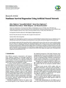
0=g(x,r,u). Where x are the state variables; r are the algebraic variables; u are the control variables; f are the non linear functions that describe the differential equations of dynamic devices models; g are the non linear functions that describe the algebraic equations of electrical network and some device models. Once equation (1) is solved through step by step integration, the status of the system can be determined from the time response of all the variables. In this study the purpose is to calculate the CCT by observing its electromechanical angular and voltage swings during simulation time. In order to do this, the test system in Fig 1 is modeled using DIgSILENT software package. The generator is modeled in 6th order with automatic voltage regulator. The parameters of the model are given in appendix A. CCT which happens to be critical in this paper was calculated in the same environment. The CCT determination of the proposed SMIB is first and foremost calculated through the time domain simulation. This is done by trial and error. The sampled data is generated by applying a single contingency (three phase fault) to line 2 on the test system at different distance. The generation is kept constant. Each sample is determined based on the behavior of the generator rotor angle. Eight fault locations are considered in this paper. The faults are located at 30, 40, 50, 60, 70, 80, 90 and 100 percent from the bus 2. The real power of the generator is 100MW and the reactive power is 80MVAR which are kept constant. After each application of fault the fault is clear by removing the line. The fault is applied at 0.1 second on line 2 and the fault is clear by removing the line at 0.15second. The value of CCTTDS is recorded in table I.

II. MATHEMATICAL MODEL OF A SINGLE MACHINE INFINITE BUS SYSTEM. The dynamics of power system model can be represented by linear and non linear equations involving many discrete and continuous state variables with sophisticated models. The equation is to be solved by time domain simulation or direct energy method [11]. For a given disturbance, the simulation program alternatively solves the non linear equations representing the dynamics of the generators, and algebraic power flow equations representing the algebraic equations. The non linear algebraic- differential equations sets are represented as: ẋ = f( x,r,u) (1)

FIG 1 Single machine infinite bus bar.

68


number of outputs compared and the error calculated. The network is also updated and the process continues again. Training stops each time the training time elapses or when the number of epoch is reached. Also whenever the error reaches acceptable level, the training stops. The whole exercise can be done as many times as possible until the desire target is reached. Another important thing is the training style which is either batch or incremental depending on the way of presentation of the input. In incremental training, the weights and biases of the network are updated each time an input is presented to the network. In batch training the weights and biases are only updated after all the inputs are presented [12]. For LM, it only allows the use of batch training style and can only be invoked by ‘TRAIN’ as against ‘ADAPT’ in incremental.

Table I: Fault location and critical clearing time (CCTTDS). FAULTS

FAULT LOCATION FROM BUS 2 (%)

FAULT LOCATION IN KM

CCT (TDS)

F1

30

186

0.56

F2

40

248

0.57

F3

50

310

0.62

F4

60

372

0.63

F5

70

434

0.64

F6

80

496

0.66

F7

90

558

0.69

F8

100

620

0.70

IV.

IMPLEMETATION OF ANN IN CCT DETERMINATION.

A. Data preparation and features selection. A large number of input/output data patterns are generated either from historical stored data or from perturbing the system randomly in a wide range of loading states. In this paper, input/ output pattern is generated by applying three phase fault based on different point on the line. Faults were applied at eight different locations on the line (F1-F8). They are 30%, 40%, 50%, 60%,70%, 80%,90% and 100% Power flow is used to initialize the state variable before commencing the time domain simulation. The simulation was run for 20 seconds with integration time step of 0.01 second. The critical clearing time was calculated by shifting the FCT to the critical point where a further increase in the time ends up being unstable. Data for each fault location are collected in which 100 sampled data were taken 0.1 second after clearing the fault. The selected features which are considered important for the determination of CCT are rotor angle, generator speed, and active power, reactive power and terminal voltage. Eight locations were considered which gives a size of 8x100 or 800 data for eight features. The total data collected is 800 x 5. The selection of input fault is an important factor to be considered in the ANN implementation. As the size of power system increases the number of input features considerably increases. So it is important to reduce the number of input features so as to minimize the training time, memory requirement and the number of weight factors during training.

III MULTI LAYER FEED FORWARD (MLFF) NEURAL NETWORKS.

Multi layer feed forward neural networks consists of several layers of neurons with one layer as output layer and others as hidden layers. It can solve more sophisticated problems than single layer net. The number of neuron of the output and hidden layers and their transfer functions are related to how the problem is defined. Input vector is fed to the input layer from the input data, the weight and the biases are adjusted using the activation function. The training is done by feeding in the training data as well as the target data. This network is normally train by back propagation algorithm. Standard back propagation is a gradient descent algorithm in which the network weights are moved along the negative of the gradient of the performance function. The gradient is computed for nonlinear multilayer networks. There are a number of variations on the basic algorithm that are based on other standard optimization techniques, such as conjugate gradient, Newton methods and Levenberg –Marquardt (LM). LM gives a good exchange between the speed of the Newton algorithm and the stability of the steepest descent methods [11]. Reference [11] shows the possibility of improving this algorithm in order to improve the speed and reduce error of oscillation. In general, the performance index is minimized in order to achieve The algorithm progresses iteratively minimum error. through a number of epochs. On each epoch the training cases are each submitted to the network and target and

B Architecture of the ANN The multi-layer feed-forward NN, also known as the multilayer perceptron (MLP) NN, is use in this work. It is characterised by its architecture, activation functions, training and learning algorithm. Figure 2 shows the simple multi-layer feed forward NN. It consists of an input layer, output layer, and one or more hidden layers. The output

69


and the hidden unit may have bias. The bias is denoted by bj and bk. Data from the input layer flow through the hidden layer to the output layer. The layers are interconnected by communication links represented as weight. The weights are determined by training algorithm. One of the popular training algorithms for the MLP NN is the error back propagation algorithm, which is based on the gradient descent technique for error reduction. In this paper, we used the MATLAB neural network toolbox to train the MLP NN with back-propagation technique. The weight and biases are adjusted iteratively to achieve a minimum mean square error between the network output and target value.

Input layer

hidden layer

bk

(4) Where wji are the weight in the output layer, wki are the weight of hidden layer. bk and bj are the bias in the hidden and output layer respectively. Pi are input values, xi are the input to the output layer C.

The collected data is divided into training, testing and validation subsets. This is randomly split into 60% training, 20% testing and 20% validation. Matlab toolbox is used as a computing tool to implement the ANN [12]. Levenberg-Marquardt is used as a training algorithm because it gives a fast convergence and better performance. The performance of TSA using the trained ANN is done by calculating the mean square error (MSE) between the estimated CCT ( CCTANN) and the target CCT ( CCTTDS).

output layer

bj

p1

V. p2

Training and performance evaluation.

RESULTS AND DISCUSSION

y In this section the results obtained from ANN for determination of CCT are presented. The CCTTDS is analytically compared with CCT ANN. The performance is evaluated by time, MSE and CCT. The mean square error is mathematically given in (5).

pn wji pn i

wki

i= 1--------------n

MSE =

.

(5)

Where p represents the number of input- output training pairs, tp is the target output for the p-th training, op is the output of the ANN. The MSE for the training and testing are given in table II. The regression analysis can also be used to indicate the overall performance of this model in CCT determination. The output of regression model is

Fig2: Architecture of multi-layer- feed forward ANN The activation function translates the output of the neuron to its input. Some of the common one are threshold, piecewise linear, sigmoid, tangent hyperbolic and Gaussian function.

(6) y is the output vectors, X is the data matrix, w is the parameter vector andd is the error vector. The impact of increasing the hidden neuron on the time of simulation is also investigated as recorded in table II. Increasing the size of the hidden neuron is expected to enhance its ability to absorb the behavior of the given system. The more the hidden neuron the lesser the error. With many hidden units used the convergence is improved with provision for local generalization [13]. The greatest challenge is the training time. Initially the training time decreases with increases number of hidden neuron, until an optimal number of hidden units is reached then it starts to decrease. From table II it shows that the optimal number of hidden units appropriate for determination of CCT is 40.

The output of the output layer is

(2) The output of the hidden layer is

(3) The output of the entire system is (2 & 3)

70


The regression analysis shown in figure 4A and 4B indicate best fit line for training, validation and testing. From this graph, the value of the CCTANN was obtained.

Table II. TEST RESULTS OF ANNs NUMBER OF HIDDEN NEURON

20

30

40

PERFORMANCE

0.001330

0.001275

0.001209

REGRESSION(TRAI NING)

8.60517e1

8.77028e1

REGRESSION(TES TING)

8.69810e1

MSE(TRAINING)

MSE(TESTING)

50

70

100

0.001208

0.001291

0.001383

8.63489-1

8.76684e1

8.7899e-1

8.60437e1

8.38908e1

8.370e-1

8.51526e1

8.12610e1

8.57273e1

1.35004e3

1.25202e3

1.37449e3

1.28627e3

1.18298e3

1.14723e3

1.311918 e-3

1.45587e3

1.48967e3

1.48371e3

1.67543e3

1.35998e3

ITERATION

46

29

18

30

13

11

TIME

0.06

0.05

0.04

0.06

0.08

0.10

(a)

(b)

Fig 4A: Regression analysis: (a) Training (b) testing,,

More time is needed to train network with 100 hidden neurons. It converges faster and the mean square error has improved. When the results of the CCT were compared, it was found that the proposed ANN can correctly determine the value of the critical clearing time with minimum mean square error. Zero mean square error indicates that there is no error. In the result presented in this paper the minimum square error during training is 1.37449e-3 with 40 hidden units and 800 x5 sampled data. Out of this 20% sampled data was randomly chosen for the testing. The result is reasonable because of the following reasons.

The test error and the validation set error have similar characteristic (Fig 3). The best validation occurs at iteration 8 and there seem to be no significant over fitting at this point (Fig 3).

Fig 4B: Regression analysis: (c) Validation,

When comparing the CCTTDS with CCTANN it was found that the CCT based on ANN was correctly predicted (table III). Table III: The comparison of CCTTDS AND CCTANN.

The final mean square error is small (Fig 4A and B).

Smooth network response indicates smaller weight and biases with low probability of over fitting.

Fig 3 PERFORMANCE OF ANN

71

Faults

CCTTDS

CCTANN

F1

0.56

0.57

F2

0.57

0.57

F3

0.62

0.62

F4

0.63

0.63

F5

0.64

0.64

F6

0.66

0.66

F7

0.69

0.69

F8

0.70

0.70


[4]

C.Pothisarm, S. Jiriwibhakom, “Critical clearing time determination EGAT system using artificial neural networks. Proc. IEEE Power Engineering Society General Meeting, Vol 2, , pp731-736, 2003. [5] K.K. Sanyal “Transient stability Assessment Using Neural Network. IEEE international conference on electric utility Deregulation, Restructuring and power technologies, Hong Kong, Vol 2,pp 633-637,2004. [6] N.Amjady, S. F.Majedi “Transient Stability Prediction by a Hybrid Intelligent system. IEEE Trans. On Power Systems, Vol. 22, No3, Aug., 2007. [7] W.p.Ferreria, Mariamdo carmo,Anna, “Transient stability analysis of electric energy system via a fuzzy ARTARTMAP”, Electric power system research, vol. 76, pp466475, April, 2006. [8] S.Krishna and K.R Padiyar “Transient Stability Assessment Using Neural Networks. Proceedings of IEEE International conference on industrial technology, Vol 2,pp627-632,2000. [9] S .Ye, Y. Zheng, Q. Qian, “Transient stability Assessment of power System Based on support Vector Machine” doi:10.2991/iske.2007.143. [10] R.Ebrahimpour, E K. Abharian “An improved method in Transient stability Assessment of power system using committee neural networks, IJCSNS international Journal of computer science and network security, vol. 9, No 1, Jan 2009. [11] A.A. Suratgar, M.B.Tavakoli, A.Hoseinabadi “Modified Levenberg- Marquardt Method for Neural Networks Training” World academy of science, Engineering and Technology 6 pp. 46-48, 2005, [12] M.A. Natick. “Neural networks toolbox for use with SIMULINK, user’s guide, The Math Works Inc 2009. [13] S. Chen, C.F.N. Cowan and P.M. Grant, “orthogonal least squares learning algorithm for radial basis function networks, IEEE Trans. Neural Networks, 2: 302-309.

VI. CONCLUSION. The application of ANN to determine CCT based on variation of fault location was compared with its time domain calculation. The implementation of the idea was tested on SMIB. It can be concluded based on the above results that optimal number of hidden units is identified to be 40. After which the training time start to increase. In this work 40 hidden neurons were used. However, the proposed ANN correctly predicts CCT. There are two ways to improve the results. Firstly, increasing the number of training pattern and the other is providing a means for fast convergence of the back propagation algorithm. The first method requires more training time and is not applicable for on-line simulation. The second method will improve the time and the mean square error. The author will focus in this direction. The next direction in this work is to apply different type of faults on a bigger network. REFERENCES [1]

[2]

[3]

S.C.Savulescu “Real time stability assessment in Modern power system control centers” John Willey&Sons,Inc, Publication, 2009. S.P.Teeuwsen, “Oscillatory stability Assessment of Power System using Computational Intelligence”, PhD Thesis submitted to the University of Duisburg/Germany, 2005. Pothisam S.Jiriwibhakorn “Critical clearing time determination of EGAT system using artificial neural networks. Power Engineering society general meeting, 2003, IEEE, vol: 2 pp731-735, 2003.

APPENDIX A Table A1: Synchronous Generator parameters for stability studies Table A2: Synchronous generator parameters

Parameter Rstr Xl Xrl Xd Xq Td̍‫׳‬

Value 0.03 0.13 0 1.2 0.7 5

Tq‫׳‬ Xd′ Xq′ Td′′ Tq′′ Xd̍′′ Xq′′

5 0.3 0.25 0.04 0.05 0.22 0.25

Parameter Sbase power output Vbase Power factor Frequency

Vaule 100MVA 80MW 13.8KV 0.8 50Hz

Table A3: The transmission line parameters Table A4: Transformers (TRI)

Vbase= 230KV Sbase= 100MVA Z= [0.05+j0.436]Ω/km Y=[0.3 x 10-6] S/km. Line lengths. 620km for L1 and L2 310km for L3

Parameters Srated HV LV Frequency X/R ratio Connection

72

Vaule 130MVA 230KV 13.8KV 50 8 YN

Table A5 Loads Data

Load

Load

1

2

P(MW)

80

80

Q(MVAR)

40

40